 |
OpenSWMM Engine
6.0.0-alpha.4
Data-oriented, plugin-extensible SWMM Engine (6.0.0-alpha.4)
|
|
OpenSWMM Engine
6.0.0-alpha.4
Data-oriented, plugin-extensible SWMM Engine (6.0.0-alpha.4)
|
Snowmelt is an additional mechanism by which urban runoff may be generated. Although flow rates are typically low, they may be sustained over several days and remove a significant fraction of pollutants deposited during the winter. Rainfall events superimposed upon snowmelt baseflow may produce higher runoff peaks and volumes as well as add to the melt rate of the snow. In the context of long term continuous simulation, runoff and pollutant loads are distributed quite differently in time between the cases when snowmelt is and is not simulated. The water and pollutant storage that occurs during winter months in colder climates cannot be simulated without including snowmelt.
As part of a broad program of testing and adaptation to Canadian conditions, a snowmelt routine was placed in SWMM for single event simulation by Proctor and Redfern, Ltd. and James F. MacLaren, Ltd., abbreviated PR-JFM (1976a, 1976b, 1977), during 1974-1976. The basic melt computations were based on routines developed by the U.S. National Weather Service, NWS (Anderson, 1973). The current SWMM implementation utilizes the Canadian SWMM snowmelt routines as a starting point and extends their capabilities to model long term continuous simulations. In addition, features were added to adapt the snowmelt process to urban conditions, since the snowmelt routines used in other watershed runoff models are aimed primarily at simulation of spring melts in large river basins. The work of the National Weather Service (Anderson, 1973, 2006) as reflected in their SNOW-17 model was heavily utilized, especially for the extension to continuous simulation and the resulting inclusion of cold content, variable melt coefficients, and areal depletion.
Several hydrologic models include snowmelt computations, e.g., Stanford Watershed Model (Crawford and Linsley, 1966), HSPF (Bicknell et al., 1997), NWS (Anderson, 1973, 1976), STORM (Corps of Engineers, 1977; Roesner et al., 1974), SSARR (Corps of Engineers, 1971), and PRMS (Leavesley et al., 1983). Useful summaries of snowmelt modeling techniques are available in texts by Eagleson (1970), Gray (1970), Fleming (1975), Linsley et al. (1975), Bedient et al. (2013), and Viessman and Lewis (2003). All of these draw upon the classic work, Snow Hydrology, of the Corps of Engineers (1956).
A review of snowmelt components of urban drainage models has been performed by Semádeni-Davies (2000). Three models were reviewed in some detail: SWMM (version 4), MouseNAM (Danish Hydraulic Institute, 1994), and HBV (Bergström, 1976; Lindström et al., 1997). Semádeni-Davies (2000) concludes that urban snowmelt routines (including those in SWMM) have been adapted directly from models developed for rural situations and therefore may not represent urban conditions well. Degree-day methods are used in all three models that she reviewed, and only limited information is available regarding coefficients in urban areas. Plowing and piling of snow in urban areas, and the change in the nature of its albedo and density are also important considerations, for which SWMM includes options for their representation. Overall, SWMM appears to be no better – and no worse – than the other two models reviewed. The descriptions of SWMM snowmelt algorithms that follow do not reflect any general improvements recommended by Semádeni-Davies (2000).
SWMM treats all snow depths as "depth of water equivalent" to avoid specification of the specific gravity of the snow pack, which is highly variable with time. The specific gravity of new snow is of the order of 0.09; an 11:1 or 10:1 ratio of snow pack depth to water equivalent depth is often used as a rule of thumb. With time, the pack compresses until the specific gravity can be considerably greater, to 0.5 and above. In urban areas, lingering snow piles may resemble ice more than snow with specific gravities approaching 1.0. Although snow pack heat conduction and storage depend on specific gravity, sufficient accuracy may be obtained without involving specific gravity. It is adequate to maintain continuity through the use of depth of water equivalent. Most input parameters are in units of inches or mm of water equivalent (in w.e., or mm w.e.). For all internal computations, conversions are made to feet of water equivalent.
Snowfall rates are determined directly from precipitation inputs by using a dividing temperature SNOTMP. If the current air temperature is at or below SNOTMP, the precipitation falls as snow. Otherwise it falls as rain. In natural areas, a surface temperature of 34° to 35°F (1-2°C) provides the dividing line between equal probabilities of rain and snow (Eagleson, 1970; Corps of Engineers, 1956). However, this separation temperature might need to be somewhat lower in urban areas due to warmer surface temperatures.
Precipitation gages tend to produce inaccurate snowfall measurements because of the complicated aerodynamics of snowflakes falling into the gage. Snowfall totals are generally underestimated as a result, by a factor that varies considerably depending upon gage exposure, wind velocity and whether or not the gage has a wind shield. The program includes a multiplier for each Rain gage object, the Snow Catch Factor (SCF), which adjusts for these effects. The SCF is only applied when precipitation falls as snow.
Although it will vary considerably from storm to storm, SCF acts as a mean correction factor over a season in the model. Anderson (1973) provides typical values of SCF as a function of wind speed, as shown in Figure 6-1, which may be helpful in establishing an initial estimate. The value of SCF can also be used to account for other factors, such as losses of snow due to interception and sublimation not accounted for in the model. Anderson (1973) states that both losses are usually small compared to the gage catch deficiency.
As discussed in Section 2.3, air temperature data is supplied to a SWMM data set from either a user-generated time series or from a climate file. If a time series is used, the entries represent instantaneous temperature readings at given points in time. Linear interpolation is used to obtain temperature values for times that fall in between those recorded in the time series. If a climate file is used, then a continuous record of maximum and minimum daily temperatures is provided. The sinusoidal interpolation method described in Section 2.4 is used to obtain an instantaneous value at any point in time during a day based on the day's max-min values. (Any missing days in the record are filled in with the max-min values from the previous day).
During the simulation, melt is generated at each time step using a degree-day type equation during dry weather and a heat balance equation during rainfall periods. The latter equation makes an adjustment for wind speed (higher melt rates at higher wind speeds). The input of wind speed data to the program was discussed in Section 2.4. There are two options: 1) as average values for each month of the year, or 2) as daily values from the same climate file used to supply daily max-min temperatures. Should wind speed data not be available, the adjustment to the melt equation is simply ignored.
The coefficients used in the degree-day melt equation vary sinusoidally, from a maximum on June 21 to a minimum on December 21. In addition, a record of the cold content of the snow is maintained. Thus, before melt can occur, the pack must be "ripened," that is, heated to a specified base temperature. Specified, constant areas of each subcatchment may be designated as snow covered, or, following the practice of melt computations in natural basins, "areal depletion curves" may be used to describe the spatial extent of snow cover as the pack melts. For instance, shaded areas would be expected to retain a snow cover longer than exposed areas. Thus, the snow covered area of each subcatchment changes with time during the simulation. Melt, after routing through the remaining snow pack, is combined with rainfall to form the spatially weighted "effective rainfall" for overland flow routing.
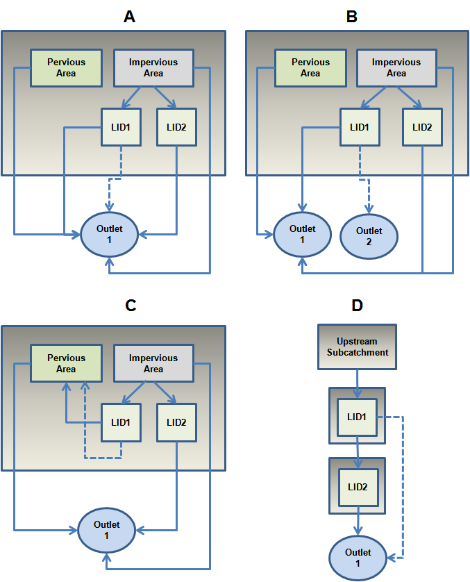
Figure 6-1 Typical gage catch deficiency correction (Anderson, 2006, p. 8).
Just as it was convenient to partition a subcatchment into three distinct areas for computing runoff (a pervious area and impervious areas both with and without depression storage – see Section 3.2), the same is true for snowmelt. The partitioning is made to facilitate the modeling of both snow removal (i.e. plowing) operations and the areal depletion phenomenon. It uses the same fractions of pervious and total impervious areas as for runoff, but instead of dividing the impervious area on the presence or absence of depression storage, it does so based on snow removal capability. That is, one fraction of the impervious area can be subjected to snow removal but not areal depletion while the reverse is true for the remaining fraction. Streets, sidewalks, and parking lots would fall into the first category, which can be considered almost normally bare of snow. Rooftops would better fit the second. Figure 6-2 illustrates the subcatchment partitioning used for snowmelt and compares it with the one used for runoff.
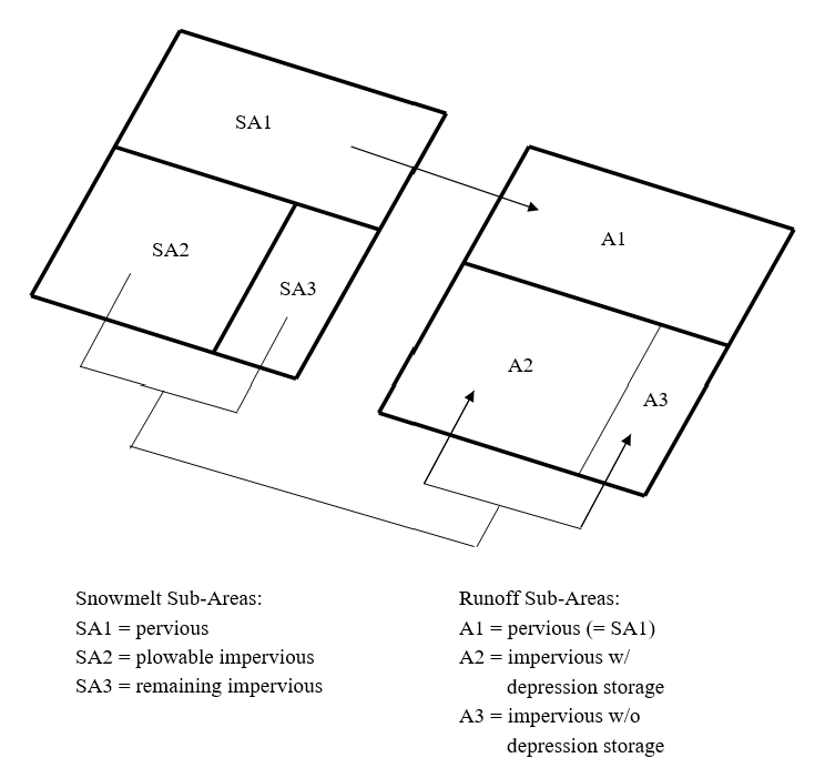
Figure 6-2 Subcatchment partitionings used for snowmelt and runoff.
A separate accounting is kept for snow accumulation and melting from each of these fractions (pervious, plowable impervious, and remaining impervious). After snowmelt calculations are made at the start of each time step, the net precipitation over the plowable and remaining impervious areas are summed together and then, for the purpose of computing runoff, are re-distributed between the fractions of impervious areas with and without depression storage. Because the pervious areas for runoff and snowmelt are the same, the snowmelt result over this sub-area can be used directly for computing pervious area runoff.
Snow removal practices form a major difference between the snow hydrology of urban and rural areas. Much of the snow cover may be completely removed from heavily urbanized areas, or plowed into windrows or piles, with melt characteristics that differ markedly from those of undisturbed snow. Management practices in cities vary according to location, climate, topography and the storm itself; they are summarized in Table 6.1. It is probably not possible to treat them all in a simulation model. However, provision is made to simulate approximately some of these practices.
A snow pack tends to insulate the surface beneath it. If ground has frozen prior to snowfall, it will tend to remain so, even as the snow begins to melt. Conversely, unfrozen ground is generally not frozen by subsequent snowfall. The infiltration characteristics of frozen versus unfrozen ground are not well understood and depend upon the moisture content at the time of freezing. For these and other reasons, SWMM assumes that snow has no effect on infiltration or other parameters, such as surface roughness or detention storage (although the latter is altered in a sense through the use of the free water holding capacity of the snow). In addition, all heat transfer calculations cease when the water becomes "net runoff". Thus, water in temporary surface storage during the overland flow routing will not refreeze as the temperature drops and is also subject to evaporation beneath the snow pack.
It is assumed that all snow subject to "redistribution", (e.g., plowing) resides on a user-specified fraction of the total impervious area (area SA2 in Figure 6-2) that might consist of streets, sidewalks, parking lots, etc. (The desired degree of definition may be obtained by using several subcatchments, although a coarse schematization, e.g., one or two subcatchments, may be sufficient for some continuous simulations.) The following five parameters, which can vary by subcatchment, govern how snow is removed or re-distributed from this sub-area:
*Fimp*: fraction of current snow transferred to the remaining impervious sub-area (SA3)
*Fperv*: fraction of current snow transferred to the pervious area (SA1)
*Fsub*: fraction of current snow transferred to the pervious area of another designated subcatchment.
*Fout*: fraction of current snow transferred out of the watershed
*Fimelt*: fraction of current snow converted into immediate melt
An instantaneous redistribution of the current snow depth begins when the latter exceeds the user-supplied parameter WEPLOW.
*Fimp* or *Fperv* are used if snow is usually windrowed onto adjacent impervious or pervious areas. If it is trucked to the pervious area of another subcatchment, the fraction *Fsub* will so indicate, or *Fout* can be used if the snow is removed entirely from the simulated watershed. In the latter case, such removals are tabulated and included in the final continuity check. Finally, excess snow may be immediately "melted" (i.e., treated as rainfall), using Fimelt. The five fractions can sum to less than 1.0 in which case some residual snow will remain on the surface. See Table 6-1 for guidelines on typical levels of service for snow and ice control (Richardson et al., 1974). The snow redistribution process does not account for snow management practices that use chemicals, such as roadway salting. This is handled using the melt equations, as described subsequently.
No pollutants are transferred with the snow. The transfers listed above are assumed to have no effect on pollutant washoff and regeneration. In addition, all the redistribution parameters remain constant throughout the simulation and can only represent averages over a snow season.
Excellent descriptions of the processes of snowmelt and accumulation are available in several texts and simulation model reports and in the well-known 1956 Snow Hydrology report by the Corps of Engineers. The important heat budget and melt components are mentioned briefly here; any of the above sources may be consulted for detailed explanations. A brief justification for the techniques adopted for snowmelt calculations in SWMM is presented below.
Table 6-1 Guidelines for level of service in snow and ice control (Richardson et al., 1974)
| Road Classification | Level of Service | Snow Depth to Start Plowing (Inches) | Max. Snow Depth on Pavement (Inches) | Full Pavement Clear of Snow After Storm (Hours) | Full Pavement Clear of Ice After Storm (Hours) |
|---|---|---|---|---|---|
| Low-Speed Multilane Urban Expressway | Roadway routinely patrolled during storms All traffic lanes treated with chemicals All lanes (including breakdown lanes) operable at all times but at reduced speeds Occasional patches of well sanded snow pack Roadway repeatedly cleared by echelons of plows to minimize traffic disruption Clear pavement obtained as soon as possible | 0.5 to 1 | 1 | 1 | 12 |
| High Speed 4-Lane Divided Highways; Interstate System; ADT greater than 10,000a | Roadway routinely patrolled during storms Driving and passing lanes treated with chemicals Driving lane operable at all times at reduced speeds Passing lane operable depending on equipment availability Clear pavement obtained as soon as possible | 1 | 2 | 1.5 | 12 |
| Primary Highways; Undivided 2 and 3 lanes; ADT 500-5000a | Roadway is routinely patrolled during storms Mostly clear pavement after storm stops Hazardous areas receive treatment of chemicals or abrasive Remaining snow and ice removed when thawing occurs | 1 | 2.5 | 2 | 24 |
| Secondary Roads ADT less than 500a | Roadway is patrolled at least once during a storm Bare left-wheel track with intermittent snow cover Hazardous areas are plowed and treated with chemicals or abrasives as a first order of work Full width of road is cleared as equipment becomes available | 2 | 3 | 3 | 48 |
aADT – average daily traffic
Snowpack Heat Budget
Heat may be added or removed from a snowpack by the following processes:
The terms may be summed, with appropriate signs, and equated to the change of heat stored in the snowpack to form a conservation of heat equation. All of the processes listed above vary in relative importance with topography, season, climate, local meteorological conditions, etc., but items 1-4 are the most important. Item 5 is of less importance on a seasonal basis, and item 6 is often neglected. A snow pack is termed "ripe" when any additional heat will produce liquid runoff. Rainfall (item 5) will rapidly ripen a snowpack by release of its latent heat of fusion as it freezes in subfreezing snow, followed by quickly filling the free water holding capacity of the snow.
Melt Prediction Techniques
Prediction of melt follows from prediction of the heat storage of the snow pack. Energy budget techniques are the most exact formulation since they evaluate each of the heat budget terms individually, requiring as meteorological input quantities such as solar radiation, air temperature, dew point or relative humidity, wind speed, and precipitation. Assumptions must be made about the density, surface roughness and heat and water storage (mass balance) of the snow pack as well as on related topographical and vegetative parameters. Further complications arise in dealing with heat conduction and roughness of the underlying ground and whether or not it is permeable.
Several models treat some or all of these effects individually, for instance, the NWS river forecast system developed by Anderson (1976). Interestingly, under many conditions he found that results obtained using his energy balance model were not significantly better than those obtained using simpler (e.g., degree-day or temperature-index) techniques in his earlier model (Anderson, 1973). The more open and variable the condition, the better is the energy balance technique. Closest agreement between his two models was for heavily forested watersheds.
The minimal data needed to apply an energy balance model are a good estimate of incoming solar radiation, plus measurements of air temperature, vapor pressure (or dew point or relative humidity) and wind speed. All of these data, except possibly solar radiation, are available for at least one location (e.g., the airport) for almost all reasonably sized cities. Even solar radiation measurements are taken at several locations in most states. Predictive techniques are also available, for solar radiation and other parameters, based on available measurements (TVA, 1972; Franz, 1974).
Choice of Predictive Method
Two major reasons suggest that simpler, e.g., temperature-index, techniques should be used for simulation of snowmelt and accumulation in urban areas. First, even though required meteorological data for energy balance models are likely to be available, there is a large local variation in the magnitude of these parameters due to the urbanization itself. For example, radiation melt will be influenced heavily by shading of buildings and albedo (reflection coefficient) reduced by urban pollutants. In view of the many unknown properties of the snowpack itself in urban areas, it may be overly ambitious to attempt to predict melt at all! But at the least, simpler techniques are probably all that are warranted. They have the added advantage of considerably reducing the already extensive input data to a model such as SWMM.
Second, the objective of the modeling should be examined. Although it may contribute, snowmelt seldom causes flooding or hydrologic extremes in an urban area itself. Hence, exact prediction of flow magnitudes does not assume nearly the importance it has in the models of, say, the NWS, in which river flood forecasting for large mountainous catchments is of paramount importance. For planning purposes in urban areas, exact quantity (or quality) prediction is not the objective in any event; rather, these efforts produce a statistical evaluation of a complex system and help identify critical time periods for more detailed analysis.
For these and other reasons, simple snowmelt prediction techniques are incorporated into SWMM. Anderson's NWS (1973) temperature-index method is also well documented and tested, and is used in SWMM. As described subsequently, the snowmelt modeling follows Anderson's work in several areas, not just in the melt equations. It may be noted that the STORM model (Corps of Engineers, 1977; Roesner et al., 1974) also uses the temperature-index method for snowmelt prediction, in a considerably less complex manner than is programmed in SWMM.
Anderson's NWS model (1973) treats two different melt situations: with and without rainfall. When there is rainfall (greater than 0.1 in/hr or 2.5 mm/hr in the NWS model, (greater than 0.02 in/hr or 0.51 mm/hr in SWMM), accurate assumptions can be made about several energy budget terms. These are: zero solar radiation, incoming long wave radiation equals blackbody radiation at the ambient air temperature, the snow surface temperature is 32° F (0° C), and the dew point and rain water temperatures equal the ambient air temperature. Anderson combines the appropriate terms for each heat budget component into one equation for the melt rate SMELT:
\[SMELT = \left( 0.001167 + 7.5\gamma U_{A} + 0.007i \right)\left( T_{a} - 32 \right) + 8.5U_{A}(e_{a} - 0.18)\]
(6-1)
where
SMELT = melt rate (in/hr) *Ta* = air temperature (° F)
γ = psychrometric constant (in Hg/° F)
*UA* = wind speed adjustment factor (in/in Hg – hr)
i = rainfall intensity (in/hr)
*ea* = saturation vapor pressure at air temperature (in Hg).
The origin of the numerical constants found in Equation 6-1 is given by Anderson (1973), and reflect units conversions as well as U.S. customary units for physical properties. The psychrometric constant, γ, is calculated as:
\[\gamma = 0.000359P_{a}\]
(6-2)
where *Pa* is the atmospheric pressure (in Hg). The latter, in turn, is calculated as a function of elevation, z:
\[P_{a} = 29.9 - 1.02(\frac{z}{1000) + 0.0032{(\frac{z}{1000)}}^{2.4}}\]
(6-3)
where z is the average catchment elevation (ft). The wind adjustment factor, *UA*, accounts for turbulent transport of sensible heat and water vapor. Anderson (1973) gives:
\[U_{A} = 0.006U\]
(6-4)
where U is the average wind speed 1.64 ft (0.5 m) above the snow surface (mi/hr). In practice, available wind data are used and are seldom corrected for the actual elevation of the anemometer. Section 6.2.2 (as well as Section 2.6) discusses how wind data are supplied to SWMM. If no such data are available on a particular date then *UA* is set equal to 0. Finally, the saturation vapor pressure, *ea*, is given accurately by the convenient exponential approximation:
\[e_{a} = 8.1175 \times 10^{6}\exp\left( \frac{- 7701.544}{T_{a} + 405.0265} \right)\]
(6-5)
During non-rain periods, melt is calculated as a linear function of the difference between the air temperature, *Ta, and a base temperature, *Tbase, using a degree-day or temperature-index type equation:
\[SMELT = DHM\left( T_{a} - Tbase \right)\]
(6-6)
where:
SMELT = melt rate (in/hr), *Ta* = air temperature (° F)
Tbase = base melt temperature (° F)
DHM = melt coefficient (in/hr-° F)
Different values of Tbase and DHM may be used for each of the three types of snow surfaces within a subcatchment. For instance, these parameters may be used to account for street salting, which lowers the base melt temperature. If desired, rooftops could be simulated using a lower value of Tbase to reflect heat transfer vertically through the roof. Suggested values for Tbase and DHM are provided in the Parameter Estimates section (6.7) below.
During the simulation, Tbase remains constant, but DHM is allowed a seasonal variation, as illustrated in Figure 6-3. Following Anderson (1973), the minimum melt coefficient is assumed to occur on December 21 and the maximum on June 21. Parameters DHMIN and DHMAX are supplied as input for the three snowpack areas of each subcatchment, and sinusoidal interpolation is used to produce a value of DHM that is constant over each day of the year:
\[DHM = \left( \frac{DHMAX + DHMIN}{2} \right) + \left( \frac{DHMAX - DHMIN}{2} \right)\sin\left( \frac{\pi}{182}(day - 81) \right)\]
(6-7)
where
DHMIN = minimum melt coefficient, occurring Dec. 21 (in/hr-°F) DHMAX = maximum melt coefficient, occurring June 21 (in/hr-°F)
day = number of the day of the year.
No special allowance is made for leap year. However, the correct date (and day number) is maintained.
height="2.8125in" height="2.8125in" height="2.8125in" height="2.8125in" height="2.8125in"
Figure 6-3 Seasonal variation of melt coefficients.
During subfreezing weather, the snow pack does not melt, and heat exchange with the atmosphere can either warm or cool the pack. The difference between the heat content of the subfreezing pack and the (higher) base melt temperature is taken as positive and termed the "cold content" of the pack. No melt will occur until the cold content is reduced to zero. It is maintained in inches (or feet) of water equivalent. That is, a cold content of 0.1 in. (2.5 mm) is equivalent to the heat required to melt 0.1 in. (2.5 mm) of snow. Following Anderson (1973), the heat exchange altering the cold content within each 6-hour period is proportional to the difference between the air temperature, *Ta, and an antecedent temperature index, *ATI, indicative of the temperature of the surface layer of the snow pack. The value of ATI is updated at the start of each time step as follows:
ATI ← ATI + TIPMt (Ta - ATI) (6-8)
where *TIPMt* is given by (Anderson, 2006):
\[{TIPM}_{t} = 1 - {(1 - TIPM)}^{\mathrm{\Delta}t/6}\]
(6-9)
for a time step Δt in hours. TIPM is a 6-hour weighting factor whose value lies between 0 and 1.0. The value of ATI is not allowed to exceed Tbase, and when snowfall is occurring, ATI takes on the current air temperature.
The weighting factor TIPM is a user-supplied constant that applies over the entire watershed. It is an indication of the thickness of the "surface" layer of snow. Values less than 0.1 give significant weight to temperatures over the past week or more and would thus indicate a deeper layer than values greater than, say, 0.5, which would essentially only give weight to temperatures during the past day. In other words, the pack will both warm and cool more slowly with low values of TIPM. Anderson states that TIPM *= 0.5* has given reasonable results in natural watersheds, although there is some evidence that a lower value may be more appropriate. No calibration has been attempted on urban watersheds.
After the antecedent temperature index is calculated, the cold content COLDC is changed by an amount
\[\mathrm{\Delta}CC = RNM \times DHM \times \left( ATI - T_{a} \right) \times \mathrm{\Delta}t\]
(6-10)
where
ΔCC = change in cold content (inches water equivalent) RNM = ratio of negative melt coefficient to melt coefficient,
DHM = melt coefficient (in/hr-° F)
ATI = antecedent temperature index (°F)
Δt = time step (hr).
Note that the cold content is increased, (ΔCC is positive) when the air temperature is less (colder) than the antecedent temperature index. Since heat transfer during non-melt periods is less than during melt periods, Anderson uses a "negative melt coefficient" in the heat exchange computation. SWMM computes this simply as a fraction, RNM, of the melt coefficient, DHM. Hence, the negative melt coefficient, i.e., the product [Figure image not available in this format]*also varies seasonally. As with *TIPM, a single user-supplied value of RNM is used throughout the study area. A typical value is 0.6.
During melting periods, cold content of the pack is reduced by an amount:
\[\mathrm{\Delta}CC = - SMELT \times RNM \times \mathrm{\Delta}t\]
(6-11)
with an equal reduction made in SMELT. Thus no liquid melt actually occurs until the snow pack cold content is reduced to 0. Even then, runoff will not occur, until the "free water holding capacity" of the snow pack is filled. This is discussed subsequently. The value of COLDC is in units of inches of water equivalent over the area in question. The cold content "volume," equivalent to calories or BTUs, is obtained by multiplying by the area. Finally, an adjustment is made to Equations 6-10 and 6-11 depending on the areal extent of snow cover. This is discussed below.
The snow pack on a catchment rarely melts uniformly over the total area. Rather, due to shading, drifting, topography, etc., certain portions of the catchment will become bare before others, and only a fraction, ASC, will be snow covered. This fraction must be known in order to compute the snow covered area available for heat exchange and melt, and to know how much rain falls on bare ground. Because of year to year similarities in topography, vegetation, drift patterns, etc., the fraction, ASC, is primarily a function of the amount of snow on the catchment at a given time; this function, called an "areal depletion curve", is discussed below. These functions are used as an option to describe the seasonal growth and recession of the snow pack. For short, single event simulation, fractions of snow covered area may be fixed for the pervious and impervious areas of each subcatchment.
As used in most snowmelt models, it is assumed that there is a depth, SI, above which there will always be 100 percent cover. In some models, the value of SI is adjusted during the simulation; in SWMM it remains constant. The amount of snow present at any time is indicated by the state variable WSNOW, which is the depth (water equivalent) over each of the three possible snow covered areas of each subcatchment (see Figure 6-2). This depth is made non-dimensional by dividing it by SI for use in calculating ASC. Thus, an areal depletion curve (ADC) is a plot of WSNOW / SI versus ASC; a typical ADC for a natural catchment is shown in Figure 6-4. For values of the ratio AWESI = WSNOW / SI greater than 1.0, ASC = 1.0, that is, the area is 100 percent snow covered.
Figure 6-4 Typical areal depletion curve for natural area (Anderson, 1973, p. 3-15) and temporary curve for new snow.
Some of the implications of different functional forms of the ADC may be seen in Figure 6-5. Since the program maintains snow quantities, WSNOW, as the depth over the total area, *AT, the actual snow depth, *WS, and actual area covered, AS, are related by continuity:
\[WSNOW \times A_{T} = WS \times AS\]
(6-12)
where:
WSNOW = depth of snow over total area (inches water equivalent) *AT* = total area (ft²),
WS = actual snow depth (inches water equivalent), and
AS = snow covered area (ft²).
In terms of parameters shown on the ADC, this equation may be rearranged to read:
\[AWESI = \frac{WSNOW}{SI = \left( \frac{WS}{SI} \right)\left( \frac{AS}{A_{T}} \right) = \left( \frac{WS}{SI} \right)ASC}\]
(6-13)
This equation can be used to compute the actual snow depth, WS, from known ADC parameters, if desired. It is unnecessary to do this in the program, but it is helpful in understanding the curves of Figure 6-5. Thus:
\[WS = \left( \frac{AWESI}{ASC} \right)\ SI\]
(6-14)
Consider the three ADC curves B, C and D of Figure 6-5. For curve B, AWESI is always less than ASC; hence WS is always less than SI as shown in Figure 6-5d. For curve C, AWESI = ASC, hence WS = SI, as shown in Figure 6-5e. Finally, for curve D, AWESI is always greater than ASC; hence, WS is always greater than SI, as shown in Figure 6-5f. Constant values of ASC at 100 percent cover and 40 percent cover are illustrated in Figure 6-5c, curve A, and Figure 6-5g, curve E, respectively. At a given time (e.g., t1 in Figure 6-5), the area of each snow depth versus area curve is the same and equal to \(AWESI \times SI\), (e.g., 0.8 SI for time t1).
Curve B on Figure 6-5a is the most common type of ADC occurring in nature, as shown in Figure 6-4. The convex curve D requires some mechanism for raising snow levels above their original depth, SI. In nature, drifting provides such a mechanism; in urban areas, plowing and windrowing could cause a similar effect. A complex curve could be generated to represent specific snow removal practices in a city. However, the program uses only one ADC curve for all impervious areas (e.g., area SA3 of Figure 6-2 for all subcatchments) and only one ADC curve for all pervious areas (e.g., area SA1 of Figure 6-2 for all subcatchments). This limitation should not hinder an adequate simulation since the effects of variations in individual locations are averaged out in the city-wide scope of most continuous simulations.
The program does not require the ADC curves to pass through the origin, AWESI = ASC = 0; they may intersect the abscissa at a value of ASC > 0 in order to maintain some snow covered area up until the instant that all snow disappears (see Figure 6-4). However, the curves may not intersect the ordinate, AWESI > 0 when ASC = 0.
The preceding paragraphs have centered on the situation where a depth of snow greater than or equal to SI has fallen and is melting. (The ADC curves are not employed until WSNOW becomes less than SI.) The situation when there is new snow needs to be discussed, starting from both zero and non-zero initial cover. The SWMM procedure again follows Anderson's NWS method (1973).
Figure 6-5 Effect of snow cover on areal depletion curves.
When there is new snow and WSNOW is already greater than or equal to SI, ASC remains unchanged at 1.0. However, when there is new snow on bare or partially bare ground, it is assumed that the total area is 100 percent covered for a period of time, and a "temporary" ADC is established as shown in Figure 6-4. This temporary curve returns to the same point on the ADC as the snow melts. Let the depth of new snow be SNO, measured in equivalent inches of water. Then the value of AWESI will be changed from an initial value of AWE to a new value of SNEW by:
\[SNEW = AWE + \frac{SNO}{SI}\]
(6-15)
It is assumed that the areal snow cover remains at 100 percent until 25 percent of the new snow melts. This defines the value of SBWS of Figure 6-4 as:
\[SBWS = AWE + 0.75\left( \frac{SNO}{SI} \right)\]
(6-16)
Anderson (1973) reports low sensitivity of model results to the arbitrary 25 percent assumption. When melt produces a value of AWESI between SBWS and AWE, linear interpolation of the temporary curve is used to find ASC until the actual ADC curve is again reached. When new snow has fallen, the program thus maintains values of AWE, SBA and SBWS (Figure 6-4).
The interactive nature of melt and fraction of snow cover is not accounted for during each time step. It is sufficient to use the value of ASC at the beginning of each time step, especially with a short (e.g., one-hour) time step for the simulation.
The fraction of area that is snow covered, ASC, is used to adjust 1) the volume of melt that occurs, and 2) the "volume" of cold content change, since it is assumed that heat transfer occurs only over the snow covered area. The melt rate is computed from either of the two equations for SMELT. The snow depth is then reduced by an amount ΔWSNOW which equals:
\[\mathrm{\Delta}WSNOW = SMELT \times ASC \times \mathrm{\Delta}t\]
(6-17)
and includes appropriate continuity checks to avoid melting more snow than is there, etc.
Cold content changes are also adjusted by the value of ASC. Thus, using Equation 6-10, cold content, COLDC, is changed by an amount ΔCC given by:
\[\mathrm{\Delta}CC = RNM \times DHM \times \left( ATI - T_{a} \right) \times \mathrm{\Delta}t \times ASC\]
(6-18)
where variables are as previously defined. Again there are program checks for negative values of COLDC, etc.
Production of melt does not necessarily mean that there will be liquid runoff at a given time step since a snow pack, acting as a porous medium with a "porosity," has a certain "free water holding capacity" at a given instant in time. Conway and Benedict (1994) describe the physics of the various processes underway as melt infiltrates into a snowpack. Following PR-JFM (1976a, 1976b), this capacity is taken to be a constant fraction, FWFRAC, of the variable snow depth, WSNOW, at each time step. This volume (depth) must be filled before runoff from the snow pack occurs. The program maintains the depth of free water, FW, inches of water, for use in these computations. When [Figure image not available in this format], the snow pack is fully ripe. The procedure is sketched in Figure 6-6.
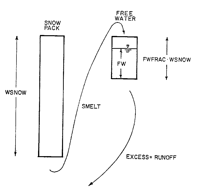
Figure 6-6 Schematic of liquid water routing through snow pack.
The inclusion of the free water holding capacity via this simple reservoir-type routing delays and somewhat attenuates the appearance of liquid runoff. When rainfall occurs, it is added to the melt rate entering storage as free water. No free water is released when melt does not occur, but remains in storage, available for release when the pack is again ripe. This re-frozen free water is not included in subsequent cold content or melt computations.
Melt from snow covered areas and rainfall on bare surfaces is area weighted and combined to produce net runoff onto the surface as follows:
\[RI = ASC \times SMELT + (1.0 - ASC) \times i\]
(6-19)
where RI is the net equivalent precipitation input onto the subcatchment surface (in/hr) and i is the liquid rainfall intensity (in/h). RI is used in place of the externally supplied rainfall value in subsequent overland flow and infiltration calculations.
If immediate melt is produced through the use of the snow redistribution fraction Fimelt it is added to the last equation. Furthermore, all melt calculations are ended when the depth of snow water equivalent becomes less than 0.001 in. (0.025 mm), and any remaining snow and free water are converted to immediate melt and added to Equation 6-19.
Snowmelt computations are a sub-procedure implemented as part of SWMM's runoff calculations. They are made at each runoff time step, for each subcatchment that has snow pack parameters assigned to it, immediately after atmospheric precipitation has been determined. This is at Step 3a of the runoff procedure described in Section 3.4. The snowmelt routine returns an adjusted precipitation rate (in/h), consisting of liquid rainfall and/or snowmelt, over each runoff sub-area of the subcatchment. These rates serve as the actual precipitation input used in the remainder of the surface runoff computation. The steps used to compute snow accumulation and snowmelt are listed in the sidebar below.
Computational Scheme for Snowmelt
The following variables are assumed known at the start of the time step of length Δt (h) for each subcatchment:
Externally supplied time series variables:
- *Ta* = air temperature (°F)
- U = wind speed (mi/h)
- i = precipitation rate (in/h)
State variables for the snow pack on each snow surface:
- WSNOW = snow pack depth (inches water equivalent)
- COLDC = cold content depth (inches water equivalent)
- FW = free water depth (inches water equivalent)
- ATI = antecedent temperature index (°F)
In addition, the following constant parameters have been supplied by the user:
Constants defined for each subcatchment assigned a Snow Pack object:
- SNN = fraction of impervious area that is plowable (i.e., SA2)
- *Tbase* = temperature at which snow begins to melt (°F)
- DHMIN = melt coefficient for December 21 (in/hr-°F)
- DHMAX = melt coefficient for June 21 (in/hr-°F)
- SI = depth at which surface remains 100% snow covered (inches)
- FWFRAC = free water fraction that produces liquid runoff from the snow pack
Snow redistribution constants for each subcatchment with a plowable sub-area SA2:
- WEPLOW = depth that initiates snow redistribution (inches)
- Redistribution fractions *Fimp*, *Fperv*, *Fsub*, *Fout*, and *Fimelt* as defined in Section 6.2.5
Constants defined for the entire study area:
- SNOTMP = dividing temperature between snowfall and rainfall (°F)
- SCF = rain gage snow capture factor (ratio)
- TIPM = ATI weighting factor (fraction)
- RNM = negative melt ratio (fraction)
- Areal depletion curves (ASC as a function of AWE) for both pervious and impervious areas
Initially (at time 0) COLDC = AWE = 0, ATI = *Tbase, and both *WSNOW and FW are user-supplied. The snowmelt computations are comprised of the following 11 steps:
- Compute the melt coefficient DHM for each snow pack surface (SA1, SA2, and SA3) for the current day of the year using Equation 6-7 and set the immediate melt IMELT on each surface to 0.
- If *Ta* ≤ SNOTMP then precipitation is in the form of snow so update the snow pack depth on each snow surface:
\[WSNOW \gets WSNOW + i \times SCF \times \Delta t\]
- For the plowable impervious snow surface (SA2), if WSNOW > WEPLOW then WSNOW is reduced to reflect the redistributions produced by the fractions *Fimp*, *Fperv*, *Fsub*, *Fout*, and *Fimelt*. If *Fimelt* > 0 then the immediate melt for surface SA2 is set to:
\[IMELT = \frac{F_{imelt} \times WSNOW}{\Delta t}\]
- If the snow pack depth over a snow surface is below 0.001 inches then convert the entire pack for that surface into immediate melt:
\[IMELT \gets IMELT + \frac{WSNOW + FW}{\Delta t}\]
and reset the pack's state variables to 0.- Use the Areal Depletion Curves supplied for the pervious (SA1) and non-plowable impervious (SA3) snow surfaces to compute a new areal snow coverage ratio ASC for these surfaces (ASC for the plowable impervious surface is always 1.0). The details are supplied below.
- Compute a snowmelt rate SMELT for the snow pack on each surface:
- If rain is falling (*Ta* > SNOTMP and i > 0.02 in/h) use the heat budget equation, Equation 6-1, converted from a 6-hour to a 1-hour time base.
- Otherwise, if *Ta* ≥ *Tbase, use the degree-day equation, Equation 6-6.
- Otherwise set *SMELT to 0.
- Multiply SMELT by its respective surface's ASC value to account for any areal depletion.
- For each snow pack surface, if SMELT is 0, then update the pack's cold content as follows:
- If snow is falling (*Ta* ≤ SNOTMP and i > 0), set ATI to *Ta. Otherwise set *ATI to the smaller of *Tbase* and the result of Equation 6-8.
- Use Equation 6-10 with the updated ATI value to compute Δ*CC* and add Δ*CC* × ASC to COLDC.
- Limit COLDC to be no greater than 0.007 WSNOW(*Tbase* - ATI) which assumes a specific heat of snow of 0.007 inches water equivalent per °F.
- For each snow pack surface under melting conditions (SMELT > 0) reduce both the cold content COLDC and the melt rate SMELT for each snow surface as follows:
\[\Delta CC = SMELT \times RNM \times \Delta t\]
\[COLDC \gets COLDC - \Delta CC\]
\[SMELT \gets SMELT - \Delta CC\]
limiting both COLDC and SMELT to be ≥ 0.- Update the snow depth and free water content of the snow pack on each snow surface:
\[WSNOW \gets WSNOW - SMELT \times \Delta t\]
\[FW \gets FW + (SMELT + i_{RAIN}) \Delta t\]
where *iRAIN* = i if precipitation falls as rain or 0 otherwise.- Check each snow surface to see if the free water content is high enough to produce liquid runoff, i.e., if FW ≥ FWFRAC × WSNOW then set:
\[\Delta FF = FW - FWFRAC \times WSNOW\]
\[FW \gets FW - \Delta FF\]
\[SMELT = \Delta FF\]
Otherwise set SMELT = 0.- Compute the overall equivalent precipitation input RI (in/h) for each snow surface as:
\[RI = SMELT + IMELT + i_{RAIN} \times (1 - ASC)\]
Use these values to return an adjusted precipitation rate i (in/h) to each of the sub-areas used to compute runoff:
- i = RI[SA1] for the pervious area A1 and
- i = (RI[SA2] × *AS2* + RI[SA3] × *AS3*) / *Aimperv* for both impervious areas A2 and A3, where RI[SA*j*] is the value of RI for snow surface SA*j*, *ASj* is the area of snow surface j, and *Aimperv* is the total impervious area.
Step 5 of the snowmelt process uses Areal Depletion curves to compute the fraction of snow covered area (ASC) for both the pervious (SA1) and impervious (SA3) areas subject to areal depletion. Note that at this stage of the calculations any snow that has fallen during the time step has already been added on to the accumulated snow depth WSNOW. The scheme used to update the fraction of snow covered area is described in the sidebar below.
Computational Scheme for Snow Covered Area
There are four different cases that can arise when computing the fraction of snow covered area ASC during the snowmelt calculations at a particular time step:
Case 1: No snow accumulation
- There is no snow accumulation (WSNOW = 0). Set ASC = 0.0 and re-set AWE to 0.
Case 2: Snow accumulation exceeds threshold
- The updated snow accumulation WSNOW is greater than SI. In this case both ASC and AWE are set to 1.0.
Case 3: Snowfall during the time step
- There was snowfall during the time step (*Ta* ≤ SNOTMP and i > 0). ASC is set to 1.0 and the parameters of a temporary linear ADC are computed as follows:
- Find the AWE value for the accumulated depth at the start of the time step:
\[AWE = \frac{WSNOW_1}{SI}\]
where *WSNOW1* is the accumulated depth before the new snowfall was added on.- Use the ADC to look up the areal coverage SBA for this prior AWE value.
- Compute the relative depth SBWS at which 75% of the new snow still remains (i.e., 25% has melted):
\[SBWS = AWE + 0.75 \frac{WSNOW - WSNOW_1}{SI}\]
and save AWE, SBA, and SBWS for use with the fourth case described next.Case 4: Snow depth below threshold with no snowfall
- The accumulated snow depth WSNOW is below SI and there is no snowfall. Define AWESI as the current ratio of WSNOW to SI. Three conditions are possible:
- If AWESI < AWE the original ADC applies so set ASC to the curve value for AWESI and set AWE to 1.0.
- If AWESI ≥ SBWS the limit of the temporary ADC for new snowfall has been reached so set ASC to 1.0.
- Otherwise compute ASC from the temporary ADC as follows:
\[ASC = SBA + (1 - SBA) \frac{AWESI - AWE}{SBWS - AWE}\]
Table 6-2 summarizes the parameters used by the snowmelt routine as well as their typical range of values. The first four entries (SNOTMP, SCF, TIPM, and RNM) are system-wide parameters that apply to the entire study area. Values for the remaining parameters are specified for each snow surface within each subcatchment where snowmelt can occur. SWMM uses a Snow Pack object to bundle together a common set of these parameters that can be applied to an entire group of subcatchments. This helps reduce the amount of input that a user must provide.
Table 6-2 Summary of snowmelt parameters (in US customary units)
| Parameter | Meaning | Typical Range |
|---|---|---|
| SNOTMP | dividing temperature between snowfall and rainfall (°F) | 32 to 36 |
| SCF | rain gage snow capture factor (ratio) | 1 to 2 |
| TIPM | ATI weighting factor (fraction) | 0.5 |
| RNM | negative melt ratio (fraction) | 0.6 |
| WEPLOW | depth at which snow redistribution begins (inches) | 0.5 to 2 |
| Tbase | temperature at which snow begins to melt (°F) | 25 to 32 |
| DHMIN | melt coefficient for December 21 (in/hr-°F) | 0.001 to 0.003 |
| DHMAX | melt coefficient for June 21 (in/hr-°F) | 0.006 to 0.007 |
| SI | depth at which surface remains 100% snow covered (inches) | 1 to 4 |
| FWFRAC | free water fraction to produce liquid runoff from pack | 0.02 to 0.10 |
Snowmelt results will be sensitive to the values used for the degree-day melt coefficient DHM. In rural areas, the melt coefficient ranges from 0.03 - 0.15 in/day-°F (1.4 - 6.9 mm/day-°C) or from 0.001 - 0.006 in/h-°F (0.057 - 0.29 mm/h-°C). Gray and Prowse (1993) provide a useful summary of such equations. In urban areas, values may tend toward the higher part of the range due to compression of the pack by vehicles, pedestrians, etc. and due to reflection of radiation onto the snow from adjacent buildings (Semádeni-Davies, 2000). Most of the available data are summarized by Semádeni-Davies (2000). Bengtsson (1981) and Westerström (1981) describe results of urban snowmelt studies in Sweden, including degree-day coefficients, which range from 3 to 8 mm/°C-day (0.07 - 0.17 in/°F-day). Additional data for snowmelt on an asphalt surface (Westerström, 1984) gave degree-day coefficients of 1.7 - 6.5 mm/°C-day (0.04 - 0.14 in/°F-day). Values of Tbase will probably range between 25 and 32 °F (-4 and 0 °C). Unfortunately, few urban area data exist to define adequately appropriate modified values for Tbase and DHM, and they may be considered calibration parameters.
The value of FWFRAC will normally be less than 0.10 and usually between 0.02 - 0.05 for deep snow packs (WSNOW > 10 inches or 254 mm water equivalent). However, Anderson (1973) reports that a value of 0.25 is not unreasonable for shallow snow packs that may form a slush layer.
An additional set of parameters not listed in Table 6-2 are those used to characterize the Areal Depletion Curves (ADCs). An ADC is characterized in SWMM by providing values of ASC (fraction of area with snow cover) for snow depth ratios (ratio of depth to depth at 100% areal coverage) that range from 0.0 to 0.9 in 0.1 increments. (By definition ASC is 1.0 for a snow depth ratio of 1.0). Table 6.3 lists the points of the ADC shown previously in Figure 6-4 that is typical of natural areas. Two ADC curves, one for pervious area and one for impervious areas, are assumed to apply across the entire watershed. The curves are not required to pass through the origin, AWE = ASC = 0; they may intersect the abscissa at a value of ASC > 0 in order to maintain some snow covered area up until the instant that all snow disappears (see Figure 6-4). However, the curves may not intersect the ordinate, AWE must be greater than 0 when ASC = 0. A curve whose ASC values are all 1.0 causes the areal depletion phenomenon to be ignored.
Table 6-3 Typical areal depletion curve for natural areas
| Depth Ratio | ASC |
|---|---|
| 0.0 | 0.10 |
| 0.1 | 0.35 |
| 0.2 | 0.53 |
| 0.3 | 0.66 |
| 0.4 | 0.75 |
| 0.5 | 0.82 |
| 0.6 | 0.87 |
| 0.7 | 0.92 |
| 0.8 | 0.95 |
| 0.9 | 0.98 |
The following numerical example illustrates the dynamic nature of snow accumulation, snow melt, and subsequent runoff. A one acre, completely impervious subcatchment is modeled over an 18 day period during which temperature fluctuates between 0 and 50 °F. The simulation begins with 1 inch of snow accumulation over the subcatchment. Table 6-4 lists the relevant subcatchment and snowpack parameters, while Tables 6-5 and 6-6 list the daily temperatures and hourly precipitation, respectively, used in the simulation. The meteorological conditions are recorded data for Raleigh, NC. Neither snow removal nor areal depletion is considered.
Table 6-4 Subcatchment and snow pack parameters for illustrative snowmelt example
| Parameter | Value |
|---|---|
| Area (acres) | 1 |
| Width (ft) | 140 |
| Slope (%) | 0.5 |
| Percent Impervious | 100 |
| Roughness Coefficient | 0.01 |
| Depression Storage (in) | 0.25 |
| Minimum Melt Coefficient (in/h/°F) | 0.001 |
| Maximum Melt Coefficient (in/h/°F) | 0.006 |
| Base Temperature (Tbase) (°F) | 30 |
| Free Water Fraction (FWFRAC) | 0.05 |
| Initial Snow Depth (in) | 1.0 |
| Initial Free Water (in) | 0.2 |
| Dividing Temperature (SNOTMP) (°F) | 34 |
| ATI Weighting Factor (TIPM) | 0.5 |
| Negative Melt Ratio (RNM) | 0.6 |
| Latitude (°) | 42 |
Table 6-5 Daily temperatures for illustrative snowmelt example
| Month/Day | Maximum Temperature (°F) | Minimum Temperature (°F) |
|---|---|---|
| 1/24 | 49 | 30 |
| 1/25 | 50 | 32 |
| 1/26 | 46 | 28 |
| 1/27 | 50 | 27 |
| 1/28 | 45 | 24 |
| 1/29 | 36 | 14 |
| 1/30 | 46 | 21 |
| 1/31 | 51 | 22 |
| 2/1 | 46 | 26 |
| 2/2 | 27 | -5 |
| 2/3 | 29 | -7 |
| 2/4 | 42 | 27 |
| 2/5 | 46 | 18 |
| 2/6 | 54 | 19 |
| 2/7 | 45 | 28 |
| 2/8 | 41 | 20 |
| 2/9 | 51 | 20 |
| 2/10 | 45 | 25 |
Table 6-6 Periods of precipitation for illustrative snowmelt example
| Date | Time | Precipitation (in) |
|---|---|---|
| 01/26 | 04:00:00 | 0.26 |
| 01/29 | 18:00:00 | 0.11 |
| 01/29 | 19:00:00 | 0.01 |
| 01/29 | 20:00:00 | 0.08 |
| 02/01 | 23:00:00 | 0.02 |
| 02/02 | 00:00:00 | 0.06 |
| 02/02 | 01:00:00 | 0.08 |
| 02/02 | 02:00:00 | 0.14 |
| 02/02 | 03:00:00 | 0.19 |
| 02/02 | 04:00:00 | 0.09 |
| 02/02 | 05:00:00 | 0.01 |
| 02/02 | 22:00:00 | 0.02 |
| 02/02 | 23:00:00 | 0.06 |
| 02/03 | 00:00:00 | 0.12 |
| 02/03 | 01:00:00 | 0.22 |
| 02/03 | 02:00:00 | 0.17 |
| 02/03 | 03:00:00 | 0.05 |
| 02/03 | 12:00:00 | 0.02 |
| 02/03 | 13:00:00 | 0.00 |
| 02/03 | 14:00:00 | 0.02 |
| 02/09 | 00:00:00 | 0.01 |
| 02/09 | 01:00:00 | 0.02 |
| 02/09 | 02:00:00 | 0.00 |
| 02/09 | 03:00:00 | 0.00 |
| 02/09 | 04:00:00 | 0.00 |
| 02/09 | 05:00:00 | 0.06 |
Figures 6-7 through 6-10 show the resulting temperature, precipitation, snow depth and runoff amounts, respectively produced by SWMM for this example. The original inch of snow takes about four days to melt completely. Runoff during this time is sporadic, due to the fluctuation in temperature around the base melt temperature. The first storm event arrives just before the end of day 2 and falls mainly as snow. This bumps up the snow cover during its 3-hour duration as shown in Figure 6-9. Snow levels rise again with the arrival of the second storm during the morning of day 5, when temperatures are below freezing. By day 6, temperatures again rise above the base melt temperature (30 °F) for part of the day and the snow from the second storm is completely melted by the start of day 7. The next storm arrives at noon of day 8 and lasts for 7 hours. The runoff spike of 0.15 in/hr seen in Figure 6-10 occurs during the first hour of this event when the temperature is still above freezing. The remainder of the storm falls as snow and starts the buildup of a snow pack once again. The next two storms add onto the pack, and no melting occurs until day 10, when temperatures again rise above the base melt value for portions of the day. Runoff from the melting pack is delayed until its free water fraction is exceeded. The pack takes another 6 days to melt during which time the runoff is sporadic as the temperature fluctuates above and below the base melt level.
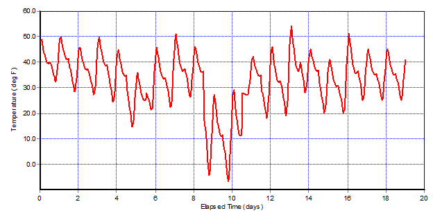
Figure 6-7 Continuous air temperature for illustrative snowmelt example.
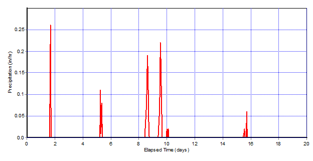
Figure 6-8 Precipitation amounts for illustrative snowmelt example.
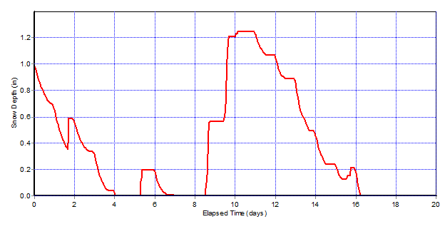
Figure 6-9 Snow pack depth for illustrative snowmelt example.
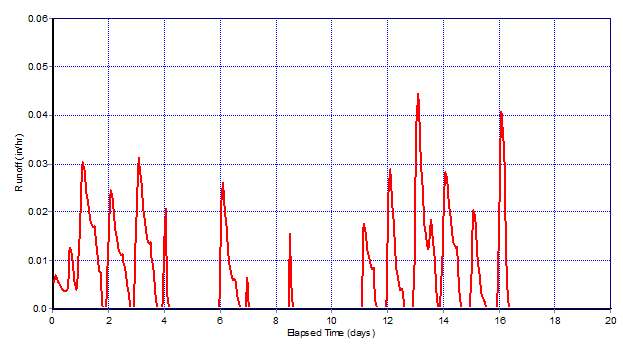
Figure 6-10 Runoff time series for illustrative snowmelt example.
 1.13.2