 |
OpenSWMM Engine
6.0.0-alpha.4
Data-oriented, plugin-extensible SWMM Engine (6.0.0-alpha.4)
|
|
OpenSWMM Engine
6.0.0-alpha.4
Data-oriented, plugin-extensible SWMM Engine (6.0.0-alpha.4)
|
Rainfall dependent (or rainfall-derived) inflow and infiltration (RDII) are stormwater flows that enter sanitary or combined sewers due to "inflow" from direct connections of downspouts, sump pumps, foundation drains, etc. as well as "infiltration" of subsurface water through cracked pipes, leaky joints, poor manhole connections, etc. RDII can be a significant cause of sanitary sewer overflows (SSOs) of untreated wastewater into basements, streets and other properties, as well as receiving streams. It can also cause significant flow increases to wastewater treatment plants resulting in hydraulic overloading and disruption of plant processes.
SWMM treats RDII as a separate category of external inflows that enters the conveyance system at specific user-designated nodes. It is computed independently of the surface runoff, infiltration, snowmelt and groundwater processes described in previous chapters of this manual. RDII flow is added onto the other inflow categories (such as dry weather sanitary flow, overland runoff, and groundwater interflow) during each time step of a simulation. RDII calculations were added to version 4 of SWMM by C. Moore of CDM in 1993. This chapter describes how these RDII flows are computed from the precipitation records supplied to a SWMM data set.
Figure 7-1 depicts the three major components of wet-weather wastewater flow within a sanitary sewer system (Vallabhaneni et al., 2007). These are base sanitary flow (BSF), groundwater infiltration (GWI), and RDII. BSF is the flow discharged to sanitary sewers by homes, businesses, institutions, and industrial water users throughout the normal course of a day. It exhibits a typical diurnal pattern, with higher flows during the morning and early evening hours and lower flows overnight. The average daily BSF remains more or less constant during the week, but can vary by both month and season.
GWI consists of groundwater that enters the collection system through cracked pipes, pipe joints and manhole walls during extended periods of time when water table levels are high, even in the absence of any rainfall. It is different from RDII because it does not occur as a direct response to a rainfall event. GWI varies throughout the year, with the highest rates in late winter and spring as groundwater levels rise, and the lowest rates (or no GWI at all) during late summer or after an extended dry period.
RDII is the flow that can be directly attributed to a rainfall event. This flow is zero before the start of the event, increases during the event, and declines back to zero sometime after the event is over. The start of the RDII response may be delayed during the time it takes for surfaces to capture a portion of the initial rainfall and for soils to become saturated. If the event is small enough, then no RDII at all may be generated. The maximum volume of rainfall that does not produce any RDII response is referred to as "initial abstraction" (Vallabhaneni et al., 2007).
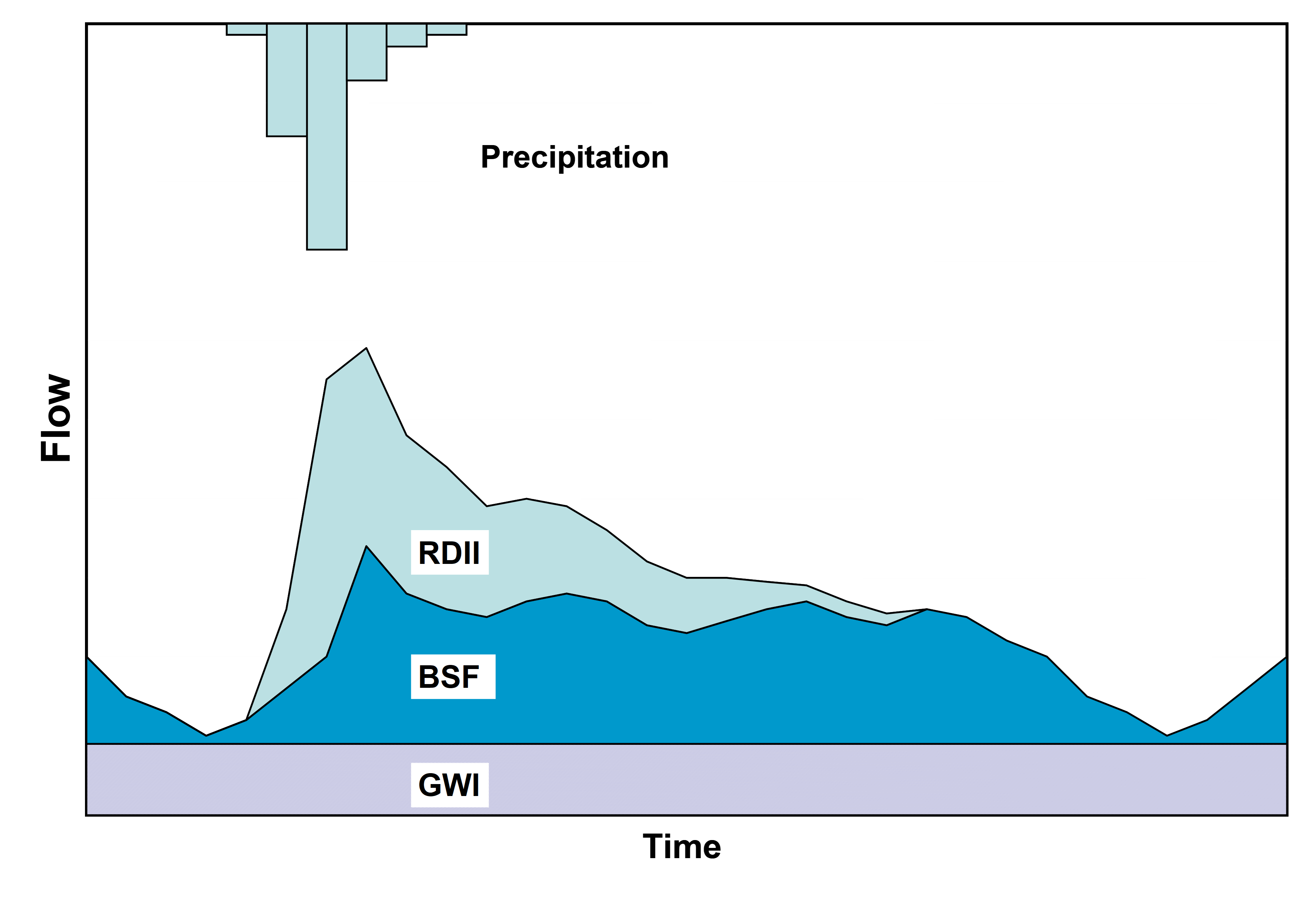
Figure 7-1 Components of wet-weather wastewater flow.
Quantitative estimates of RDII are almost always derived from actual wastewater flow records as opposed to attempting to model the distributed set of small scale physical processes directly responsible for RDII. Methods for modeling RDII are reviewed by Bennet et al. (1999) and Lai (2008). SWMM uses the RTK unit hydrograph approach, which is among the most flexible and widely used RDII methods (Vallabhaneni et al., 2007). (The initials RTK stand for the three parameters that characterize the unit hydrographs used by the method.)
The RTK unit hydrograph method was first developed by CDM-Smith consultants in an RDII study for the East Bay Municipal Utility District in Oakland, CA (Giguere and Riek, 1983). It represents the response of a sewershed to a rainfall event through a series of up to three triangular unit hydrographs. These unit hydrographs can be applied to any particular storm event to produce a resulting time history of RDII flow rates.
Figure 7-2 shows a single triangular unit hydrograph assumed to represent the RDII flow induced by one unit of rainfall over a unit of time. This unit hydrograph is characterized by the following parameters:
R: the fraction of rainfall volume that enters the sewer system and equals the volume under the hydrograph
T: the time from the onset of rainfall to the peak of the unit hydrograph
K: the ratio of time to recession of the unit hydrograph to the time to peak
*Qpeak*: peak flow (per unit area) on the unit hydrograph.
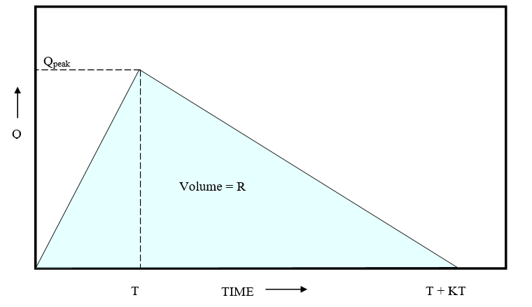
Figure 7-2 Example of an RDII triangular unit hydrograph.
Figure 7-3 shows how this single unit hydrograph would be applied to a storm that consists of three time periods of varying rainfall volume. The original unit hydrograph is replicated for each rainfall time period, with its origin offset by the time period and its ordinates multiplied by the rainfall volume for that period. The overall response to the storm is the hydrograph obtained by summing the ordinates of the volume-adjusted hydrographs at each time point. The volumetric RDII inflow into the conveyance system is the ordinate of the composite hydrograph multiplied by the contributing area of the affected sewershed. This process of adding together the rainfall-adjusted, time-shifted hydrographs is known as convolution (Chow et al, 1988) and is expressed mathematically as:
\[Q_{t} = \sum_{j = 1}^{t}{U_{t - j + 1}P_{j}}\]
(7-1)
where:
*Qt* = RDII flow per unit area during time period t, *Ut* = ordinate of the unit hydrograph for time period t,
*Pj* = depth of rainfall for time period j.
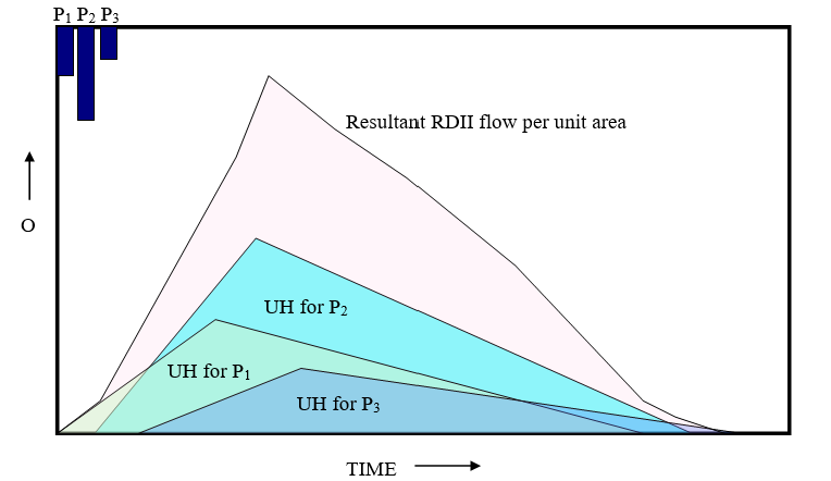
Figure 7-3 Application of a unit hydrograph to a storm event.
The ordinate value *Uj* for time period j is determined from the shape parameters R, T, and K of the unit hydrograph as follows. One can write:
\[U_{j} = f_{j}Q_{peak}\]
(7-2)
where *fj* is the fraction of the rising limb (or falling limb) that corresponds to time period j. Because the area under the unit hydrograph is R, the value of *Qpeak* is:
\[Q_{peak} = \frac{2R}{T + KT}\]
(7-3)
Thus *Uj*can be expressed as:
\[U_{j} = \frac{2Rf_{j}}{T + KT}\]
(7-4)
By convention, the time τ_j on the unit hydrograph base corresponding to time period j is taken as the midpoint between either ends of the time interval:
\[\tau_{j} = (j - 0.5)\Delta\tau\]
(7-5)
where Δτ is the time interval over which precipitation is recorded. The fraction *fj* is then determined as:
\[f_{j} = \frac{\tau_{j}}{T}\]
for τ_j ≤ T (7-6)
\[f_{j} = 1 - \frac{\tau_{j - T}}{KT}\]
for T < τ_j ≤ T + KT (7-7)
\[f_{j} = 0\]
for τ_j > T + KT (7-8)
Because actual RDII hydrographs have complex shapes, three different hydrographs of increasing durations are typically used to represent the overall RDII unit response (Vallabhaneni et al., 2007). The first hydrograph models the most rapidly responding inflow component usually caused by direct sources of inflow, and has a time to peak T of one to three hours. The second includes both rainfall-derived inflow and infiltration, and has a longer T value. The third represents infiltration that may continue long after the storm event has ended and has the longest T value. Figure 7-4 depicts how the three unit hydrographs are summed together to produce a total RDII hydrograph in response to a unit of rainfall over one unit of time. Equation 7-1 is still used to compute the overall RDII hydrograph to any given storm event, with a separate *Qt* computed for each of the three unit hydrographs. These are then added together to produce the total flow per unit area for time period t.
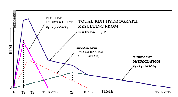
Figure 7-4 Use of three unit hydrographs to represent RDII (Vallabhaneni et al., 2007).
Not all storms will result in measurable inflow/infiltration. Just as with ordinary runoff, a certain initial volume of rainfall will be captured by surface ponding, interception by flat roofs and vegetation, and surface wetting and will not contribute to RDII. This phenomenon is represented in SWMM by three user-supplied "initial abstraction" (IA) parameters that accompany each RDII unit hydrograph. *IAmax* (in or mm) is the maximum depth of initial abstraction capacity available for the sewershed. *IA0* (in or mm) is the amount of that capacity already used up at the start of the simulation. *IAr* (in/day or mm/day) is the rate at which capacity becomes available again during periods of no rainfall. During storm events, the volume of rainfall applied to the unit hydrograph convolution formula, Equation 7-1, is reduced by the amount of initial abstraction capacity remaining. During dry periods, this capacity is regenerated based on the user-supplied recovery rate.
SWMM generates RDII inflows for specific nodes of a sewer system. Recall from Section 1.2 that SWMM uses a network of links and nodes to represent the conveyance portion of a drainage area. For RDII applications this network would be the sewer system (either sanitary or combined), the links are the sewer pipes and the nodes are points where pipes connect to one another (e.g., manholes or pipe fittings).
It should be noted once again that RDII is computed independently from any surface runoff or groundwater flow generated from the subcatchments contained in a SWMM model. The sewershed that produces RDII flow for a specific sewer system node is not represented explicitly in SWMM and need not correspond to any of the runoff subcatchments defined for the study area. In fact it is perfectly acceptable (and quite common for sanitary sewer systems) to conduct an RDII analysis without including any subcatchments in the model. In this case the model would consist of a set of Rain Gage objects (and their data sources), the node and link objects that make up the sewer network and sets of user-supplied time series that describe groundwater (GWI) and sanitary (BSF) flows.
SWMM computes all RDII inflow time series prior to the start of a simulation and saves these inflow values to an interface file. Each line of the file contains, in chronological order, a node ID name, a date, a time of day, and the RDII inflow value for that node. Dates with no RDII inflows are not recorded. To compute the entries of this file the following quantities are assumed known for each node of the conveyance system node that receives RDII inflows:
The steps used to process a precipitation record against a set of unit hydrographs to produce a record of RDII inflows for a specific conveyance node are described in the sidebar shown below.
To use SWMM's RDII option a user must supply estimates of the three parameters (R, T, and K) that define each of three unit hydrographs for each node where RDII enters the sewer system. Each unit hydrograph can also have a set of initial abstraction parameters (Ia_0, Ia_max, and Ia_r). SWMM also allows one to specify different sets of unit hydrographs and initial abstraction parameters for different months of the year. In addition, the area of the RDII contributing sewershed must also be specified.
When the [HYDROGRAPHS] section supplies more than one set of parameters for the same month and response (short-, medium- or long-term) of a unit hydrograph group, the values read last are the ones used and warning message 13 is issued. In particular, an ALL entry assigns its values to every month, so an ALL entry that follows month-specific entries silently replaces them (and vice versa — month-specific entries appearing after an ALL entry replace the ALL values for those months). Models that mix ALL and month-specific entries for the same response should therefore order them deliberately and heed the warning. This check is performed in RDIISolver::init() (src/engine/hydrology/RDII.cpp; see openswmm::rdii::RDIISolver).
R-T-K parameters are derived from site-specific flow monitoring data. There are no general values that can be applied in the absence of actual field data. All of these parameters require that a continuous flow monitoring program be implemented at strategic points in the sewer system. As described in Vallabhaneni et al., 2007, estimating the RDII unit hydrograph parameters for a sewershed involves the following activities:
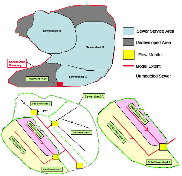
Figure 7-5 Sewershed delineation (Vallabhaneni et al., 2007).
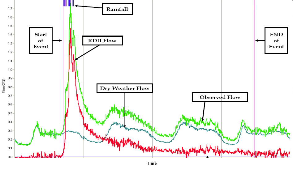
Figure 7-6 Extracting RDII flow from a continuous flow monitor (Vallabhaneni et al., 2007).
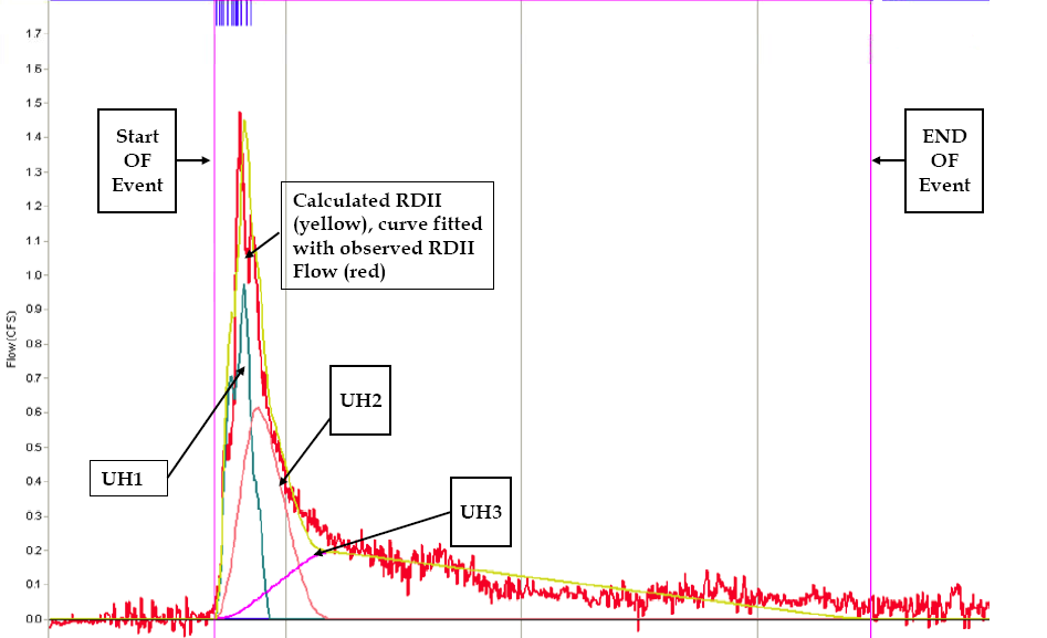
Figure 7-7 Fitting unit hydrographs to an RDII flow record (Vallabhaneni et al., 2007).
A simple example illustrates how SWMM constructs an RDII interface file for use within a hydraulic simulation. Assume there is a single rain gage whose rainfall time series is shown in Table 7-1. Note that the recording interval is 1 hour, and that there are two events separated by 22 hours. SWMM will use data from this gage to construct a time series of RDII flows for a node named N1 in the conveyance system that services an area of 10 acres. There is a single group of 3 unit hydrographs used to derive RDII from the rain gage data. The shapes and parameters of the unit hydrographs (UH1, UH2, and UH3) are shown in Figure 7-8. Note that the R-values of this set of unit hydrographs sum to 0.36, implying that 36 percent of total rainfall volume winds up as RDII. To keep things simple, initial abstraction is not considered in this example.
Table 7-1 Rainfall time series for the illustrative RDII example
| Hour | Rainfall (inches) |
|---|---|
| 0:00 | 0.0 |
| 1:00 | 0.25 |
| 2:00 | 0.5 |
| 3:00 | 0.8 |
| 4:00 | 0.4 |
| 5:00 | 0.1 |
| 6:00 | 0.0 |
| 27:00 | 0.0 |
| 28:00 | 0.4 |
| 29:00 | 0.2 |
| 30:00 | 0.0 |
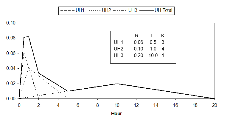
Figure 7-8 Unit hydrographs used for the illustrative RDII example.
The resulting RDII flows are depicted in Figure 7-9. SWMM places these flows into an RDII interface file, a portion of which is displayed in Figure 7-10. This file is accessed during the flow routing portion of a SWMM run to add RDII inflow into node N1 at each time step of the routing process.
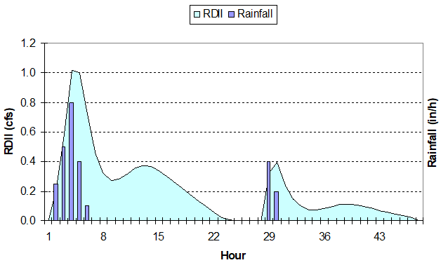
Figure 7-9 Time series of RDII flows for the illustrative RDII example.
SWMM5 Interface File
| Node | Year | Mon | Day | Hr | Min | Sec | FLOW |
|---|---|---|---|---|---|---|---|
| N1 | 2002 | 02 | 02 | 01 | 15 | 00 | 0.204195 |
| N1 | 2002 | 02 | 02 | 01 | 30 | 00 | 0.204195 |
| N1 | 2002 | 02 | 02 | 01 | 45 | 00 | 0.204195 |
| N1 | 2002 | 02 | 02 | 02 | 00 | 00 | 0.204195 |
| N1 | 2002 | 02 | 02 | 02 | 15 | 00 | 0.554604 |
| N1 | 2002 | 02 | 02 | 02 | 30 | 00 | 0.554604 |
| N1 | 2002 | 02 | 02 | 02 | 45 | 00 | 0.554604 |
| N1 | 2002 | 02 | 02 | 03 | 00 | 00 | 0.554604 |
| N1 | 2002 | 02 | 02 | 03 | 15 | 00 | 1.021479 |
| N1 | 2002 | 02 | 02 | 03 | 30 | 00 | 1.021479 |
| N1 | 2002 | 02 | 02 | 03 | 45 | 00 | 1.021479 |
| N1 | 2002 | 02 | 02 | 04 | 00 | 00 | 1.021479 |
| N1 | 2002 | 02 | 02 | 04 | 15 | 00 | 1.001312 |
| N1 | 2002 | 02 | 02 | 04 | 30 | 00 | 1.001312 |
| N1 | 2002 | 02 | 02 | 04 | 45 | 00 | 1.001312 |
| N1 | 2002 | 02 | 02 | 05 | 00 | 00 | 1.001312 |
| N1 | 2002 | 02 | 02 | 05 | 15 | 00 | 0.703842 |
| N1 | 2002 | 02 | 02 | 05 | 30 | 00 | 0.703842 |
| N1 | 2002 | 02 | 02 | 05 | 45 | 00 | 0.703842 |
| N1 | 2002 | 02 | 02 | 06 | 00 | 00 | 0.703842 |
Figure 7-10 Excerpt from the RDII interface file for the illustrative RDII example.
The initial abstraction model described in Section 7.2 depletes the available abstraction capacity linearly with rainfall depth and restores it at a constant user-supplied rate *IAr* during dry weather, independent of season or temperature. In practice, RDII response varies strongly through the year: in winter and early spring the soil surrounding sewer infrastructure is near saturation, abstraction capacity is depleted, and a large fraction of rainfall reaches the pipe; in summer and autumn evapotranspiration has dried the soil, capacity is restored, and the same storm produces far less RDII. With the linear model this seasonal variation must be imposed externally by calibrating different R values for each month, which conflates two distinct physical quantities — the infrastructure leakage fraction, a property of pipe condition that should not vary seasonally, and the antecedent moisture state, a dynamic variable that evolves with the weather. A model calibrated this way cannot represent an anomalously wet summer or dry winter and does not transfer to altered climate conditions.
As an alternative, SWMM offers an exponential-decay initial abstraction model in which the abstraction capacity is depleted exponentially with rainfall depth and recovers exponentially at a temperature-dependent rate. Seasonal variation in RDII response then emerges from the tracked moisture state acting on a single, seasonally invariant set of R-T-K values, rather than from calendar-month lookup tables. The model is enabled per unit hydrograph group and per response (short-, medium- or long-term) so that adoption can be incremental; responses without exponential-decay parameters continue to use the linear model of Section 7.2.
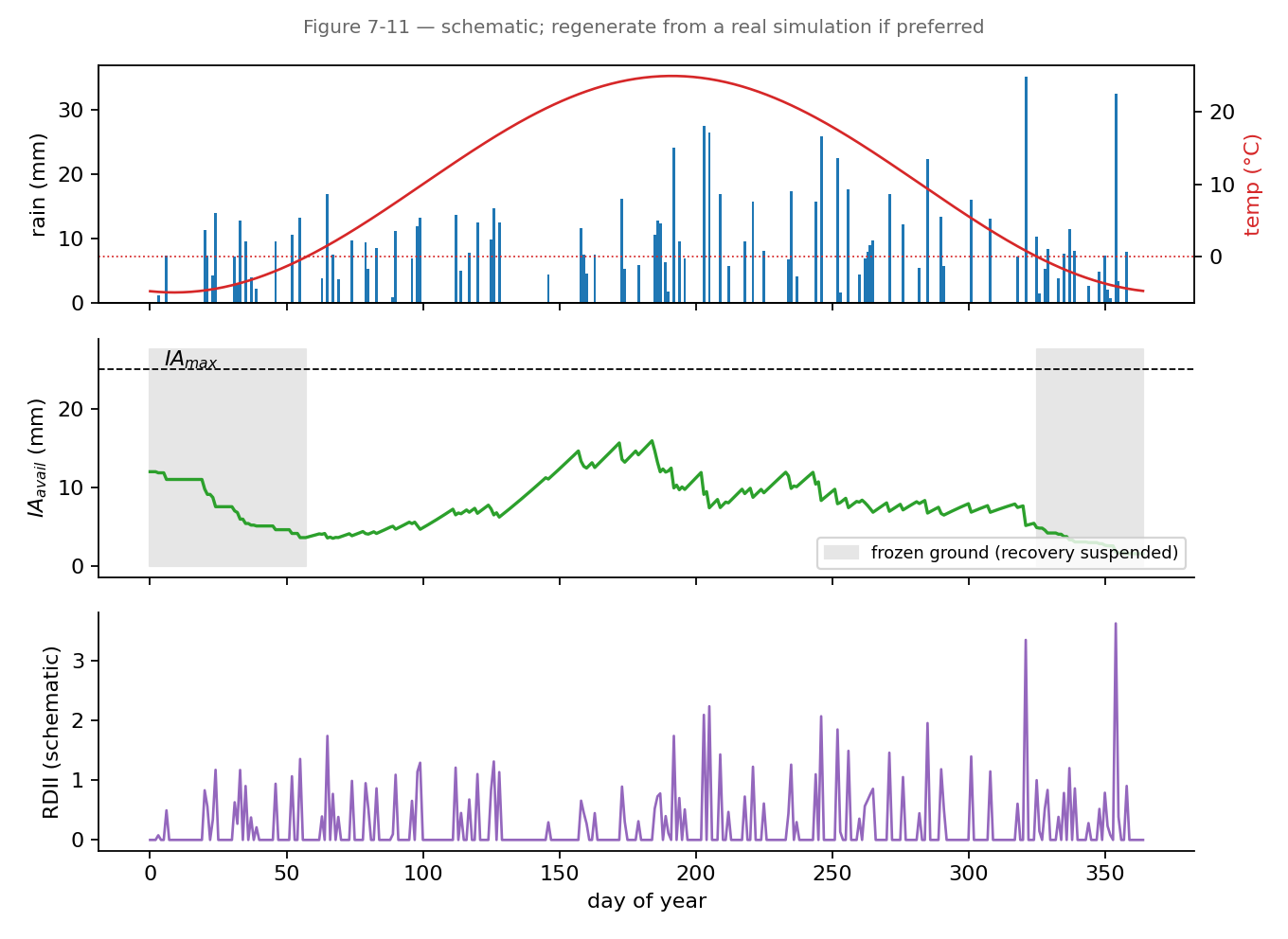
Figure 7-11 Emergent seasonal behavior of the exponential-decay initial abstraction model (schematic, synthetic forcing): available initial abstraction depletes during storms, recovery is suspended on frozen ground and accelerates in warm months, and a single R-T-K set produces a seasonally varying RDII response.
Let *IAavail* denote the available (unused) abstraction capacity, bounded between 0 and *IAmax. During time steps with rainfall, the available capacity decays exponentially with the rainfall depth *ΔP accumulated over the step:
\[IA_{avail}^{t + \Delta t} = IA_{avail}^{t}\ e^{- k_{dep}\Delta P}\]
(7-9)
where *kdep* is a depletion rate coefficient with units of inverse rainfall depth (1/in for US units, 1/mm for SI units). The depth abstracted from the rainfall is exactly the depth removed from the storage, and the rainfall excess passed to the unit hydrograph convolution of Equation 7-1 is:
\[P_{net} = \max\left( 0,\ \Delta P - \left( IA_{avail}^{t} - IA_{avail}^{t + \Delta t} \right) \right)\]
(7-10)
This mass-consistent bookkeeping — the storage drains by the same depth it abstracts — is essential to the model's behavior. Note two limiting cases: *kdep* = 0 disables abstraction entirely (the excess equals the rainfall and the state never changes), while a very large *kdep* consumes the full remaining capacity on any rainfall. A rule of thumb for an initial estimate is *kdep* ≈ 1/*IAmax*.
During dry time steps the available capacity recovers toward *IAmax* according to the first-order rate equation:
\[\frac{d\ IA_{avail}}{dt} = k_{rec}(T)\left( IA_{max} - IA_{avail} \right)\]
(7-11)
which is integrated exactly over the time step as:
\[IA_{avail}^{t + \Delta t} = IA_{max} - \left( IA_{max} - IA_{avail}^{t} \right)e^{- k_{rec}(T)\Delta t}\]
(7-12)
The asymptotic approach to *IAmax* is physically realistic — recovery is fast when the deficit is large and slows as capacity is restored — in contrast to the constant-rate recovery of the linear model. The recovery rate coefficient *krec* (1/hr) is the sum of a temperature-independent base rate and a thermally activated rate, with recovery suppressed entirely on frozen ground:
\[k_{rec}(T) = \begin{cases} 0 & T < T_{freeze} \\ k_{0} + k_{T}\ e^{\theta_{rec}\left( T - T_{ref} \right)} & T \geq T_{freeze} \end{cases}\]
(7-13)
where T is the current air temperature (deg C), *k0* (1/hr) represents gravity drainage and capillary redistribution that proceed regardless of temperature, *kT* (1/hr) is the evapotranspiration-driven recovery rate at the reference temperature *Tref* (deg C), *θrec* (1/deg C) is the temperature sensitivity of the thermal term, and *Tfreeze* (deg C) is the threshold below which frozen or near-frozen ground suppresses all recovery. The additive form guarantees a minimum recovery rate *k0* even in cool conditions above freezing, and centers the thermal term so that *krec* = *k0* + *kT* exactly when T = *Tref*. A convenient choice for *Tref* is the mean annual air temperature of the study area. The frozen-ground suppression reproduces the elevated early-spring RDII observed in cold-climate systems: abstraction deficit accumulated during autumn storms persists through winter without recovery, so effective capacity entering spring is low.
Air temperature is obtained from the project's temperature data source (Section 2.3). If no temperature source is configured, the model evaluates *krec* at *Tref* for every step — recovery still occurs but produces no seasonal variation — and a warning is issued at the start of the simulation.
Near full capacity, a first-order expansion of Equation 7-12 reduces to the linear model of Section 7.2 with an effective recovery rate *IAr* = *krec(T)·(IAmax − IAavail)*, so the exponential formulation is a generalization that converges to the linear model for small deficits and diverges — correctly — under large deficits and long dry periods.
Because RDII is computed independently of the subcatchment snowmelt model of Chapter 6, sewersheds in cold climates would otherwise treat winter snowfall as immediately available rainfall. The exponential-decay model therefore offers an optional degree-day snow partition applied to the precipitation before the depletion and recovery calculations. When the air temperature is at or below a threshold *Tsnow* (deg C), precipitation accumulates as snow water equivalent (SWE) and provides no liquid input for that step. When the temperature is above the threshold and SWE is present, melt is released at a degree-day rate and added to any concurrent rainfall (rain-on-snow):
\[M = \min\left( SWE,\ DDF\left( T - T_{snow} \right)\Delta t \right)\]
(7-14)
where M is the melt depth released during the step, DDF is the degree-day melt factor (in/deg C/day for US units, mm/deg C/day for SI units), and Δt is the step length in days. A DDF of zero with the snow partition enabled is an accumulate-only configuration: cold-period precipitation is withheld from the abstraction model and never melts. The snow partition requires a temperature data source to be meaningful; if none is configured a warning is issued, since the temperature is then fixed at *Tref* and either all precipitation becomes permanent snowpack (if *Tref* ≤ *Tsnow*) or the snow parameters have no effect.
Exponential-decay parameters are supplied in a [RDII_DECAY] section, one line per unit hydrograph group and response:
where UHGroup is a unit hydrograph group name from the [HYDROGRAPHS] section, Response is one of SHORT, MEDIUM or LONG, and the literal keyword SNOW followed by *Tsnow* and DDF enables the optional snow partition of Section 7.6.3. The parameters are summarized in Table 7-2. Lines with negative *kdep*, *k0*, *kT* or DDF values are ignored.
Table 7-2 Parameters of the [RDII_DECAY] section
| Parameter | Units | Description |
|---|---|---|
| *kdep* | 1/in (US) or 1/mm (SI) | Depletion rate per unit depth of rainfall (Equation 7-9) |
| *k0* | 1/hr | Base recovery rate, independent of temperature |
| *kT* | 1/hr | Thermal recovery rate at the reference temperature |
| *Tref* | deg C | Reference temperature for the thermal recovery term |
| *θrec* | 1/deg C | Temperature sensitivity of the thermal recovery term |
| *Tfreeze* | deg C | Temperature below which all recovery is suppressed |
| *Tsnow* | deg C | Optional rain/snow partition threshold and melt base temperature |
| DDF | in/deg C/day (US) or mm/deg C/day (SI) | Optional degree-day melt factor |
The [HYDROGRAPHS] section is unchanged. When a [RDII_DECAY] line is present for a given group and response, the linear recovery rate *IAr* from [HYDROGRAPHS] is ignored for that response, while *IAmax* and *IA0* continue to be used since they describe the abstraction reservoir itself rather than its dynamics. A group with no [RDII_DECAY] lines uses the linear model for all three responses; a group with one line falls back to the linear model for the two unspecified responses. Because the tracked moisture state supplies the seasonal variation, a single ALL entry per response in [HYDROGRAPHS] is normally sufficient when exponential decay is active. The simulation status report identifies which formulation is in effect ("Exponential IA" versus "Linear IA").
In addition to the missing-temperature-source warnings noted above, warnings are issued at the start of a run for degenerate configurations: *kdep* = 0 (abstraction disabled, recovery parameters without effect) and *Tfreeze* ≥ *Tref* (recovery suppressed at the reference temperature).
The runtime state of the exponential model is the same used-abstraction depth tracked by the linear model, so hot start files written under either formulation initialize the other correctly.
The exponential-decay model is preferable for continuous, multi-year simulations in which seasonal RDII variation matters — the situation where the linear model forces monthly R calibration. It is particularly suited to cold-climate systems with a spring RDII peak (through the frozen-ground and snow-partition mechanisms), to climate scenario analysis (since the calibrated R-T-K parameters are seasonally invariant properties of the infrastructure and transfer to altered temperature records), and to studies of antecedent moisture effects such as back-to-back storms. For single-event design simulations, or when re-using an existing model already calibrated with monthly parameters, the classical linear model remains appropriate and is the default.
When migrating a model calibrated with monthly R values, the minimum R across months (the driest antecedent condition) approximates the true infrastructure leakage fraction and can be adopted as the single invariant R; the spread between the maximum and minimum monthly R values indicates how much seasonal moisture effect the abstraction parameters must reproduce. Table 7-3 lists typical parameter ranges as starting points for calibration; *k0* is best estimated from inter-event recovery in cool-season storm pairs (where evapotranspiration is negligible), *kT* from the additional recovery seen in warm-season pairs, and *θrec* from seasonal residuals of multi-year records (set *θrec* = 0 when only single-season data are available).
Table 7-3 Typical parameter ranges for the exponential-decay model
| Parameter | Typical range | Physical interpretation |
|---|---|---|
| *kdep* | 1.3 – 7.6 (1/in); 0.05 – 0.30 (1/mm) | Abstraction exhaustion rate per unit depth of rainfall |
| *k0* | 0.005 – 0.03 (1/hr) | Gravity drainage and capillary redistribution |
| *kT* | 0.005 – 0.12 (1/hr) | Evapotranspiration-driven drying at *Tref* |
| *Tref* | Mean annual temperature | Anchor point for *kT* |
| *θrec* | 0.03 – 0.10 (1/deg C) | Seasonal sensitivity; 0 for isothermal recovery |
| *Tfreeze* | 0 deg C | Frozen-ground recovery threshold |
Implementation. The exponential depletion and recovery of Equations 7-9 through 7-13 are implemented in updateIA_exp() and getRecoveryRate() in src/engine/hydrology/RDII.cpp, with the linear model of Section 7.2 in updateIA_linear(); the per-response dispatch between the two occurs in RDIISolver::computeAll() (see openswmm::rdii::RDIISolver and openswmm::rdii::ExpDecayParams). Startup validation warnings are issued by RDIISolver::validateExpDecay(). The [RDII_DECAY] section is parsed by handle_rdii_decay() in src/engine/input/handlers/InflowsHandler.cpp and stored in openswmm::RDIIDecayData (src/engine/data/InflowData.hpp).
 1.13.2