1.1 What is SWMM?

The EPA Storm Water Management Model (SWMM) is a dynamic rainfall-runoff simulation model used for single event or long-term (continuous) simulation of runoff quantity and quality from primarily urban areas. The runoff component of SWMM operates on a collection of subcatchment areas that receive precipitation and generate runoff and pollutant loads. The routing portion of SWMM transports this runoff through a system of pipes, channels, storage/treatment devices, pumps, and regulators. SWMM tracks the quantity and quality of runoff generated within each subcatchment, and the flow rate, flow depth, and quality of water in each pipe and channel during a simulation period comprised of multiple time steps.

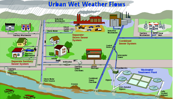
Figure 1-1. A schematic diagram showing the generation and fate of urban wet weather flows.

#user_manual_figure1_1 #user_manual_figure1_1 #user_manual_figure1_1 #user_manual_figure1_1 #user_manual_figure1_1

SWMM was first released in 1971 and has undergone several major upgrades since then. It continues to be widely used throughout the world for planning, analysis and design related to storm water runoff, combined sewers, sanitary sewers, and other drainage systems in urban areas, with many applications in non-urban areas as well. The current edition, Version 5, is a complete re-write of previous releases.

Running under Windows, SWMM 5 provides an integrated environment for editing study area input data, running hydrologic, hydraulic and water quality simulations, and viewing the results in a variety of formats. These include color-coded drainage area and conveyance system maps, time series graphs and tables, profile plots, and statistical frequency analyses.

OpenSWMM 6.0 represents a major architectural overhaul of the engine, re-implemented in C++20 with a clean plugin-extensible design. It introduces the openswmm Python package, which provides first-class programmatic access to all simulation capabilities. See Chapter 13 for a full description of the new engine and Python API.

1.2 Modeling Capabilities

SWMM accounts for various hydrologic processes that produce runoff from land surfaces. These include:

time-varying rainfall
evaporation of standing surface water
snow accumulation and melting
rainfall interception from depression storage
infiltration of rainfall into unsaturated soil layers
percolation of infiltrated water into groundwater layers
interflow between groundwater and the drainage system
nonlinear reservoir routing of overland flow
rainfall-dependent infiltration and inflow (RDII) for sanitary sewersheds
capture and retention of rainfall/runoff with various types of low impact development (LID) practices.

Spatial variability in all of these processes is achieved by dividing a study area into a collection of smaller, homogeneous subcatchment areas, each containing its own fraction of pervious and impervious subareas. Overland flow can be routed between subareas, between subcatchments, or between entry points of a drainage system.

SWMM also contains a flexible set of hydraulic modeling capabilities used to route runoff and external inflows through a drainage system network of pipes, channels, storage/treatment units and diversion structures. These include the ability to:

handle networks of unlimited size
use a wide variety of standard closed and open conduit shapes as well as natural channels
model special elements such as storage/treatment units, curb and gutter inlets, culverts, flow dividers, pumps, weirs, and orifices
apply external flows and water quality inputs from surface runoff, groundwater interflow, rainfall-dependent infiltration and inflow, dry weather- sanitary flow, and user-defined inflows
utilize either kinematic wave or full dynamic wave flow routing methods
model various flow regimes, such as backwater, surcharging, reverse flow, and surface ponding
apply user-defined dynamic control rules to simulate the operation of pumps, orifice openings, and weir crest levels.

In addition to modeling the generation and transport of runoff flows, SWMM can also estimate the production of pollutant loads associated with this runoff. The following processes can be modeled for any number of user-defined water quality constituents:

dry-weather pollutant buildup over different land uses
pollutant washoff from specific land uses during storm events
direct contribution of rainfall deposition
reduction in dry-weather buildup due to street cleaning
reduction in washoff load due to BMPs
entry of dry weather sanitary flows and user-specified external inflows at any point in the drainage system
routing of water quality constituents through the drainage system
reduction in constituent concentration through treatment in storage units or by natural processes in pipes and channels.

1.3 Typical Applications of SWMM

Since its inception, SWMM has been used in thousands of sewer and stormwater studies throughout the world. Typical applications include:

design and sizing of drainage system components for flood control
sizing of detention facilities and their appurtenances for flood control and water quality protection
flood plain mapping of natural channel systems
designing control strategies for minimizing combined sewer overflows
evaluating the impact of rainfall-dependent infiltration and inflow on sanitary sewer overflows
generating non-point source pollutant loadings for waste load allocation studies
evaluating the effectiveness of BMPs for reducing wet weather pollutant loadings.

1.4 Installing EPA SWMM

EPA SWMM 5.3 runs on both 32- and 64-bit versions of Microsoft Windows. It is distributed as a single file named swmm52#(x86)_setup.exe for the 32-bit edition or swmm52#(x64)_setup.exe for the 64-bit edition (where # is the current release number which as of this writing is 0) that contains a self-extracting setup program. To install EPA SWMM:

Select the Search icon from the Windows Taskbar and enter the word Run.
In the Run dialog that appears click the Browse button to locate the SWMM setup file on your computer.
Click the OK button type to begin the setup process.

The setup program will ask you to choose a folder (directory) where the SWMM program files will be placed. After the files are installed your Start Menu will have a new item named EPA SWMM 5.2.# where # is the current release number. To launch SWMM, select this item off of the Start Menu, and then select SWMM 5.2 from the submenu that appears. (The name of the executable file that runs SWMM under Windows is epaswmm5.exe.)

A user’s personal settings for running SWMM are stored in a folder named EPASWMM under the user’s Application Data directory (e.g., Users<username>\AppData\Roaming\EPASWMM ). If you need to save these settings to a different location, you can install a shortcut to SWMM 5 on the desktop whose target entry includes the full path name of the SWMM 5 executable followed by /s <userfolder>, where <userfolder> is the name of the folder where the personal settings will be stored. An example might be:

“c:\Program Files\EPA SWMM 5.2\epaswmm5.exe” /s “My Folders\SWMM5\”.

Several example data sets have been included with the installation package to help users become familiar with the program. They are placed in a sub-folder named EPA SWMM Projects\Sample Projects in the user’s Documents folder. Each example consists of an .INP file that holds the project’s data along with a .TXT file that describes the system being modeled.

To remove EPA SWMM from your computer, do the following:

Select Settings from the Windows Start menu.
Select Apps from the Settings page.
Select EPA SWMM 5.2.# from the list of programs that appears.
Click the Uninstall button.

1.5 Steps in Using SWMM

One typically carries out the following steps when using EPA SWMM to model a study area:

Specify a default set of options and object properties to use (see Section 5.4).
Draw a network representation of the physical components of the study area (see Section 6.2).
Edit the properties of the objects that make up the system (see Section 6.4).
Select a set of analysis options (see Section 8.1).
Run a simulation (see Section 8.4).
View the results of the simulation (see Chapter 9).

For building larger systems from scratch it might be more convenient to replace Step 2 by collecting study area data from various sources, such as CAD drawings or GIS files, and transferring these data into a SWMM input file whose format is described in Appendix D of this manual.

1.6 About This Manual

Chapter 2 presents a short tutorial to help get started using EPA SWMM. It shows how to add objects to a SWMM project, how to edit the properties of these objects, how to run a single event simulation for both hydrology and water quality, and how to run a long-term continuous simulation.

Chapter 3 provides background material on how SWMM models stormwater runoff within a drainage area. It discusses the behavior of the physical components that comprise a stormwater drainage area and collection system as well as how additional modeling information, such as rainfall quantity, dry weather sanitary inflows, and operational control, are handled. It also provides an overview of how the numerical simulation of system hydrology, hydraulics and water quality behavior is carried out.

Chapter 4 shows how the EPA SWMM graphical user interface is organized. It describes the functions of the various menu options and toolbar buttons, and how the three main windows – the Study Area Map, the Browser panel, and the Property Editor—are used.

Chapter 5 discusses the project files that store all of the information contained in a SWMM model of a drainage system. It shows how to create, open, and save these files as well as how to set default project options. It also discusses how to register calibration data that are used to compare simulation results against actual measurements.

Chapter 6 describes how one goes about building a network model of a drainage system with SWMM. It shows how to create the various physical objects (subcatchment areas, drainage pipes and channels, pumps, weirs, storage units, etc.) that make up a system, how to edit the properties of these objects, and how to describe the way that externally imposed inflows, boundary conditions and operational controls change over time.

Chapter 7 explains how to use the study area map that provides a graphical view of the system being modeled. It shows how to view different design and computed variables in color-coded fashion on the map, how to re-scale, zoom, and pan the map, how to locate objects by name on the map, how to utilize a backdrop image, and what options are available to customize the appearance of the map.

Chapter 8 shows how to run a simulation of a SWMM model. It describes the options that control how the analysis is made and offers some troubleshooting tips to use when examining simulation results.

Chapter 9 discusses the various ways in which the results of an analysis can be viewed. These include different views of the study area map, various kinds of graphs and tables, and several different types of special reports.

Chapter 10 explains how to print and copy the results discussed in Chapter 9.

Chapter 11 describes how EPA SWMM can use different types of interface files to make simulations runs more efficient.

Chapter 12 describes how add-in tools can be registered and share data with SWMM. These tools are external applications launched from SWMM’s graphical user interface that can extend its capabilities.

Chapter 13 introduces the OpenSWMM Engine v6 programmatic C API, which allows models to be built, run, and queried entirely through code without requiring an input file. It covers the engine lifecycle, building a network, callbacks, hot start files, Python bindings, and integration with CMake.

The manual also contains several appendixes:

Appendix A - provides several useful tables of parameter values, including a table of units of expression for all design and computed quantities.

Appendix B - lists the editable properties of all visual objects that can be displayed on the study area map and be selected for editing using point and click.

Appendix C - describes the specialized editors available for setting the properties of non-visual objects.

Appendix D - provides instructions for running the command line version of SWMM and includes a detailed description of the format of a project file.

Appendix E - lists all of the error messages and their meaning that SWMM can produce.