 |
OpenSWMM Engine
6.0.0-alpha.4
Data-oriented, plugin-extensible SWMM Engine (6.0.0-alpha.4)
|
|
OpenSWMM Engine
6.0.0-alpha.4
Data-oriented, plugin-extensible SWMM Engine (6.0.0-alpha.4)
|
Washoff is the process of erosion or dissolving of constituents from a subcatchment surface during a period of runoff. If the water depth is more than a few millimeters, erosion may be described by sediment transport theory in which the mass flow rate of sediment is proportional to flow and bottom shear stress, and a critical shear stress can be used to determine incipient motion of a particle resting on the bottom of a stream channel (Graf, 1971; Vanoni, 1975). Such a mechanism might apply over pervious areas and in street gutters and larger channels. For thin overland flow, however, rainfall energy can also cause particle detachment and motion. This effect is often incorporated into predictive methods for erosion from pervious areas (Wischmeier and Smith, 1958; Haan et al., 1994; Bicknell et al., 1997) and may also apply to washoff from impervious surfaces, although in this latter case, the effect of a limited supply (buildup) of the material must be considered.
Ammon (1979) reviewed several theoretical approaches for urban runoff washoff and concluded that although the sediment transport based theory is attractive, it is often insufficient in practice because of lack of data for parameter (e.g., shear stress) evaluation, sensitivity to time step and discretization and because simpler methods usually work as well (still with some theoretical basis) and are usually able to duplicate observed washoff phenomena. SWMM therefore incorporates three different choices of empirical models to represent pollutant washoff: exponential washoff, rating curve washoff, and event mean concentration (EMC) washoff.
The most oft-cited results for pollutant washoff behavior are those of Sartor and Boyd (1972), shown in Figure 4-1, in which constituents were flushed from streets using a sprinkler system. From the figure it would appear that an exponential relationship could be developed to describe washoff of the form:
\[W(t) = m_{B}(0)(1 - e^{- kt})\]
(4-1)
where W = the cumulative mass of constituent washed off at time t, *mB(0)* = the initial mass of constituent on the surface at time 0, and k = a coefficient.
It is clear that the coefficient, k, is a function of both particle size and runoff rate. An analysis of the Sartor and Boyd (1972) data by Ammon (1979) indicates that k increases with runoff rate, as would be expected, and decreases with particle size.
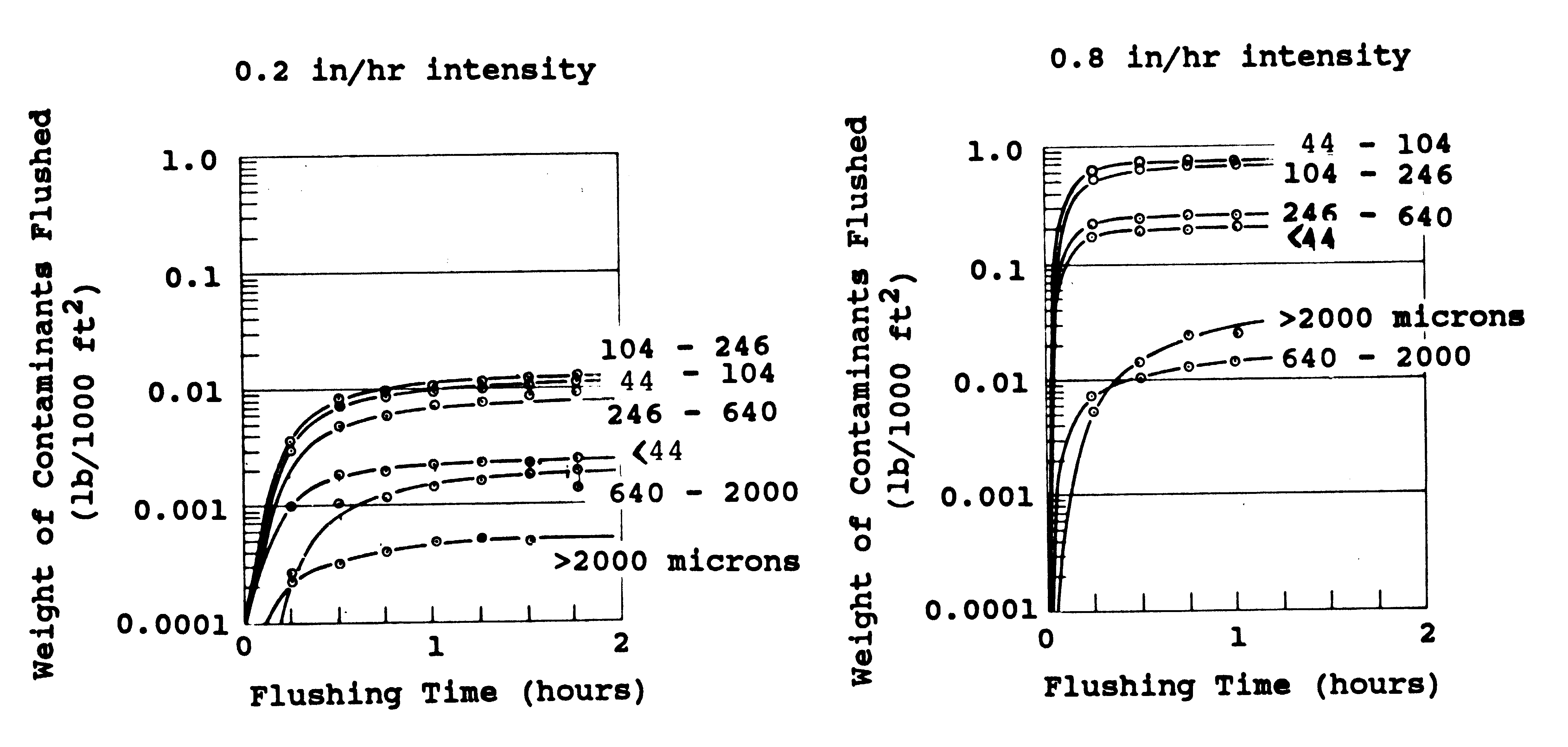
Figure 4‑1 Washoff of street solids by flushing with a sprinkler system (from Sartor and Boyd, 1972)
The Sartor and Boyd data lend credibility to the washoff assumption included in the original SWMM release (and all versions to date) that the rate of washoff, w, (e.g., mg/hr) at any time is proportional to the remaining pollutant buildup:
\[w = \frac{dm_{B}}{dt} = - km_{B}\]
(4-2)
It follows then that the amount of buildup B remaining on the surface after a time t of washoff is:
\[m_{B}(t) = m_{B}(0)e^{- kt}\]
(4-3)
This relation was first proposed by Mr. Allen J. Burdoin, a consultant to Metcalf and Eddy, during the original SWMM development. The coefficient k may be evaluated by assuming it is proportional to runoff rate:
\[k = K_{W}q\]
(4-4)
where *KW* = a washoff coefficient (in-1) and q = the runoff rate over the subcatchment (in/hr).
Burdoin assumed that one-half inch of total runoff in one hour would wash off 90 percent of the initial surface load, leading to the now familiar (in SWMM modeling circles) value of *KW* of 4.6 in.-1. (The actual time distribution of intensity does not affect the calculation of *KW.*) To the authors' knowledge, there are no direct measurements to validate this assumption, which is so often employed.
Sonnen (1980) estimated values for *KW* from sediment transport theory ranging from 0.052 to 6.6 in.-1, increasing as particle diameter decreases, rainfall intensity decreases, and as catchment area decreases. He pointed out that 4.6 in.-1 is relatively large compared to most of his calculated values. Although the exponential washoff formulation of Equations 4-2 and 4-3 is not completely satisfactory as explained below, it has been verified experimentally by Nakamura (1984a, 1984b), who also showed the dependence of the coefficient k on slope, runoff rate and cumulative runoff volume.
It was found that the original exponential washoff formulation did not adequately fit some data (Huber and Dickinson, 1988) since making k be linearly dependent on runoff rate q always produced decreasing washoff concentrations as a function of time. To see this, substitute (4-4) into (4-2) and convert the mass rate w to a concentration by dividing by the volumetric runoff rate qA, where A is the subcatchment area:
\[c = \frac{(\frac{dm_{B}}{dt})}{qA} = \frac{K_{W}qm_{B}}{qA} = \frac{K_{W}m_{B}}{A}\]
(4-5)
Thus concentration c would decrease continually as the remaining buildup *mB* does the same over time. To avoid this behavior, the relationship in (4-4) was modified to be:
\[k = K_{W}q^{N_{W}}\]
(4-6)
where *NW* is a washoff exponent. The resulting equation for exponential washoff now becomes:
\[w = K_{W}q^{N_{W}}m_{B}\]
(4-7)
with units of mass/hour.
In natural catchments and rivers, both theory and data support the result that load rate of sediment is proportional to flow rate raised to a power. For instance, sediment data from streams can usually be described by a sediment rating curve of the form
\[w = K_{W}Q^{N_{W}}\]
(4-8)
where w is sediment loading rate (mass/sec), Q is flow rate (cfs), and *KW* and *NW* are coefficients. Due to a hysteresis effect, such relationships may vary during the passing of a flood wave, but the functional form is evident in many rivers, e.g., Vanoni (1975), pp. 220-225, Graf (1971), pp. 234-241, and Simons and Senturk (1977), p.
Note the similarity of Equation 4-8 to the exponential washoff function 4-7. The presence of buildup *mB* in Equation 4-7 reflects the fact that the total quantity of sediment washed off a largely impervious urban area is likely to be limited to the amount built up during dry weather. Natural catchments and rivers from which Equation 4-8 is derived generally have no source limitation.
Also note that the form of the runoff rate used in the two functions is different. Exponential washoff uses a normalized runoff rate, q in (inches/hr), over the total subcatchment surface (both pervious and impervious areas). Rating curve washoff uses the volumetric runoff rate Q in cfs, over the fraction *fLU* of total subcatchment area A (in acres) devoted to the land use being analyzed. That is,
\[Q = qf_{LU}A\]
(4-9)
The rating curve approach may be combined with constituent buildup if desired to limit the total mass that can be washed off. Otherwise, there is no buildup between storms during continuous simulation, nor will measures like street sweeping have any effect. Constituents will be generated solely on the basis of flow rate.
If buildup is simulated when a rating curve is used, the maximum amount that can be removed is the amount built up prior to the storm. It will have an effect only if this limit is reached, at which time loads and concentrations will suddenly drop to zero. They will not assume non-zero values again until dry-weather time steps occur to allow buildup. Street sweeping will have an effect if the buildup limit is reached.
The rating curve method is generally easiest to use when only total runoff volumes and pollutant loads are available for calibration.
As a part of NPDES stormwater permitting and as a result of many special studies, there are numerous sources of local event mean concentration (EMC) data available for stormwater. EMC values are usually measured by laboratory analysis of flow- and time-weighted composite samples. EMCs are often the only samples available, in order to save on laboratory costs that would be involved in measurements of several points along the storm hydrograph, although the latter, intra-event samples are particularly valuable data. As a practical matter, EMCs are the most common parameters used to estimate nonpoint water quality loads in SWMM and in most other models. The EMC washoff function has the form:
\[w = K_{W}qf_{LU}A\]
(4-10)
where now *KW* is the EMC concentration expressed in the same volumetric units as flow rate (e.g., if the EMC is in mg/L and flow is in cfs then *KW* = EMC × 28.3 L/ft3). As with rating curve washoff, \(qf_{LU}A\) is the fraction of the total runoff rate that applies to the land use being analyzed. With EMC washoff all storms will have identical within-storm washoff concentrations. Only the loading rate will vary in direct proportion to runoff rate.
Table 4-1 lists the units of the washoff coefficient *KW* for the three different washoff models, assuming pollutant mass units of milligrams. Take note that the units of washoff rate w are mass/hr for exponential washoff and mass/sec for the other two functions. Also note that the runoff rate used in the washoff equations, whether q or Q, is based on the runoff computed for the entire subcatchment before any internal routing between the impervious and pervious sub-areas takes place (see Volume I for more details on internal runoff routing). The runoff rate actually leaving the subcatchment, which is what SWMM reports to the user, will always be a lower number when the internal routing option is used.
**Table 4‑1 Units of the washoff coefficient *KW* for different washoff models**
| Model (Washoff Units) | US Units (flow in cfs) | SI Units (flow in cms) |
|---|---|---|
| Exponential (mg/hr) | (in/hr)-NW hr-1 | (mm/hr)-NW hr-1 |
| Rating Curve (mg/sec) | (mg/sec) (cfs)-NW | (mg/sec) (cms)-NW |
| EMC (mg/sec) | mg/ft3 | mg/m3 |
Figure 4-2 compares the shapes of the runoff pollutgraphs for the three different washoff functions for an initial buildup of 20 lbs of pollutant over a one acre catchment subjected to a 2-inch, 6-hour storm with a triangular-shaped runoff hydrograph. To make the functions comparable, their coefficients were selected so that the storm would remove about 45 percent of the initial buildup. The resulting coefficient values are:
Function ***KW*** ***NW*** Exponential 0.45 (in/hr)-1.5(hr)-1 1.5
Rating Curve 850 (mg/sec)(cfs)-1.5 1.5
EMC 20 mg/L × 28.3 L/ft3 -
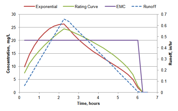
Figure 4‑2 Comparison of washoff functions
It is possible to estimate a *KW* for rating curve washoff that will produce results roughly similar to those for exponential washoff by multiplying the exponential *KW* by an average buildup seen over a storm event and converting from mass/hr to mass/sec. So for this example, assuming an average buildup of 15 lb over the event, the result is:
\[K_{W,\ RC} = 0.45 \times 15\ lb\ \times 454000\ (\frac{mg}{lb)\ \times (\frac{1}{3600)\ (\frac{hr}{sec) \approx 850}}}\]
The exponential *KW* value of 0.45 was selected by trial and error to achieve the target of removing 45 percent of the initial buildup.
In addition to the washoff of constituents deposited during dry periods, subcatchment runoff may also contain pollutant loads contributed by direct rainfall and by runon from upstream subcatchments. The instantaneous loading rates from these two streams cannot simply be added onto the loads computed from the washoff functions described earlier because they must first be routed through the volume of water (shallow as it may be) that ponds atop the surface of the subcatchment. See Volume I for a description of how SWMM uses a nonlinear reservoir model to describe surface runoff. Consistent with the way that the flow from direct rainfall and runon is treated, these pollutant streams are completely mixed with the current contents of the ponded water and a mass balance is performed to find the pollutant mass from these sources leaving the ponded surface water over the computational time step. This mass flux is added to the mass flux computed from the washoff functions to arrive at a total washoff amount.
Figure 4-3 depicts this two stream approach to handling washoff from both pollutant buildup and from rainfall/runon. A mass balance for the pollutant and volume of the washoff stream originating from the ponded surface water that receives upstream run-on and direct deposition can be written as:
\[\frac{d\left( V_{ponded}C_{ponded} \right)}{dt} = Q_{runon}C_{runon} + Q_{ppt}C_{ppt} - C_{ponded}\left( Q_{infil} + Q_{out} \right)\]
(4-11)
\[\frac{dV_{ponded}}{dt} = Q_{runon} + Q_{ppt} - Q_{infil} - Q_{evap} - Q_{out}\]
(4-12)
with the variables defined as follows:
*Vponded* = volume of water ponded over the subcatchment (ft3)
*Cponded* = concentration of pollutant in the ponded water (mg/L)
*Qrunon* = flow rate of runon onto the subcatchment (cfs)
*Crunon* = concentration of pollutant in the runon stream (mg/L)
*Qppt* = precipitation rate (cfs)
*Cppt* = concentration of pollutant in precipitation (mg/L)
*Qinfil* = infiltration rate (cfs)
*Qevap* = evaporation rate (cfs)
*Qout* = rate of runoff leaving the subcatchment (cfs).
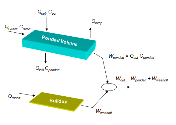
Figure 4‑3 Two-stream approach to modeling pollutant washoff
Note the following:
*Wwashoff* is the total washoff rate obtained by adding together the washoff rates w computed for the buildup on each land use. The runoff load from ponded surface storage, *Wponded*, is *Qout* *Cponded*. The total mass flow rate of pollutant leaving the subcatchment, *Wout*, is *Wwashoff* + *Wponded*. And finally, the concentration of pollutant in the subcatchment's runoff is *Wout / Qout*.
Note that this scheme requires that an additional set of state variables be kept track of over a simulation, namely the ponded mass ( \(m_{P} = V_{ponded}C_{ponded}\)) for each pollutant in each subcatchment.
Both washoff and ponded pollutant loads may be reduced by applying a BMP removal factor to them. This factor is meant to reflect the effect that some assumed best management practice (BMP) would have in removing a surface runoff pollutant. Examples of such BMPs are vegetated swales, overland flow, and riparian buffer strips. Typical removals for these practices are listed in Table 4-2.
Table 4‑2 Percent removals for vegetated swales and filter strips Source: ASCE (2001).
| Constituent | Vegetated Swales | Buffer Strips |
|---|---|---|
| Total Nitrogen | 0 – 25 | 20 – 60 |
| Total Phosphorus | 29 – 45 | 20 – 60 |
| Suspended Solids | 60 – 83 | 20 – 80 |
| Heavy Metals | 35 | 20 - 80 |
A different BMP removal factor can be associated with each pollutant and category of land use. For washoff of surface buildup, they are applied separately to the washoff rate computed for each pollutant in each land use in a given subcatchment:
\[W_{washoff} = \sum_{j}^{}{w_{jp}(1 - R_{jp})}\]
(4-13)
where *Wwashoff* is the total washoff rate (mass/sec) from buildup of pollutant p over the subcatchment, *wjp* is the washoff rate of pollutant p over land use j in the subcatchment*,* and *Rjp* is the BMP removal factor for pollutant p and land use j.
For the pollutant load from rainfall/runon across the entire subcatchment (and therefore all land uses) an area weighted average removal factor is used:
\[R_{avg,p} = \frac{\sum_{j}^{}{R_{jp}A_{j}}}{\sum_{j}^{}A_{j}}\]
(4-14)
where *Aj* is the area of land use j in the subcatchment. Thus *Wponded* for pollutant p in the subcatchment becomes:
\[W_{ponded} = Q_{out}C_{ponded}(1 - R_{avg,p})\]
(4-15)
where it is understood that *Qout* and *Cponded* refer to the pollutant and subcatchment of interest.
Pollutant washoff computations are a sub-procedure implemented as part of SWMM's runoff calculations. They are made at each runoff time step for each subcatchment immediately after surface runoff has been computed as described in Section 3.4 of Volume I. They follow a three-stage process that first computes the loading rate for each constituent due to washoff of surface buildup, then adds to that the loading rate from rainfall/runon, and finally divides the total loading rate by the runoff flow rate to arrive at a constituent concentration in the runoff leaving the subcatchment.
This first phase finds the mass flow rate of each pollutant resulting from washoff of dry deposition buildup. The following quantities are known for each subcatchment, pollutant, and user-defined land use at the start of the current time step of length ∆t:
*KW,* washoff coefficients for each pollutant – land use *NW* combination
*Rjp* BMP removal factor for each pollutant – land use combination
A subcatchment area (acres)
\(f_{LUj}\) fraction of subcatchment area occupied by each land use j
q runoff rate per unit area before any internal re-routing is made (in/hr)
\(m_{Bjp}\) mass of buildup of each pollutant p on each land use area j of the subcatchment
The computational steps for finding the washoff rate from pollutant buildup on a particular subcatchment at the current time step are:
For each combination of pollutant p and land use j do the following:
a. If the runoff rate q is less than 0.001 in/hr or if buildup is being modeled and its current value is zero then the washoff rate *wjp* = 0.
b. Otherwise use the appropriate washoff function (Equation 4-7, 4-8, or 4-10) to find the washoff rate \(w_{jp}\) for each pollutant and land use. For rating curve and EMC functions use a flow rate of \(\ Q = qf_{LUj}A\).
c. Reduce the buildup by the amount of washoff over the time step: \(m_{Bjp} = m_{Bjp} - w_{jp}\mathrm{\Delta}t\).
d. Reduce the washoff rate by the BMP removal factor: \(w_{jp} = w_{jp}(1 - R_{jp})\).
e. Add the washoff rate for this land use to the total rate *Wwashoff,p* for the subcatchment: \(W_{washoff,p} = W_{washoff,p} + w_{jp}\).
The next phase of the washoff calculations evaluates the contribution that pollutant loads in direct rainfall and upstream runon make to the total washoff load from a given subcatchment. The following quantities are known for each subcatchment and pollutant at the start of the current time step of length ∆t seconds:
*Qppt* precipitation rate over the subcatchment (cfs)
*Cppt* concentration of pollutant in precipitation (mass/ft3)
*Qrunon* rate of runon flow onto the subcatchment (cfs)
*Wrunon* rate of mass flow of pollutant in runon to subcatchment (mass/sec)
*Qout* flow rate of runoff leaving the subcatchment (cfs)
*d1* depth of ponded water over the subcatchment at the start of the time step (ft)
*d2* depth of ponded water over the subcatchment at the end of the time step (ft)
*mP* mass of ponded pollutant over the subcatchment at the start of the time step
*Ravg* area averaged BMP removal factor for the pollutant
A area of the subcatchment (ft2)
*Qppt, Qrunon, Qout*, *d1* and *d2* are known from the runoff calculation that has already been made for the current time step. *Wrunon* was also evaluated by summing the products of runoff flow and concentration from the previous time step for each of the upstream subcatchments that send their runoff to the subcatchment being analyzed.
The following steps are used to compute the rate at which pollutant mass from rainfall/runon is washed off a given subcatchment.
\[M_{Ponded} = m_{p} + (Q_{ppt}C_{ppt} + W_{runon})\mathrm{\Delta}t\]
.Note that the effects of mass lost to infiltration and volume loss due to evaporation are implicitly accounted for in step 5 where the end-of-time step volume *d2A* is used to find the mass of pollutant remaining on the subcatchment.
The final phase of the calculation adds together the two mass flow streams to arrive at a total washoff loading rate, *W~out\ ~*for the subcatchment and pollutant being analyzed:
\[W_{out} = W_{washoff} + W_{ponded}\]
(4-16)
The concentration of pollutant in the subcatchment's outflow runoff at the end of the current time step is then:
\[C_{out} = \frac{W_{out}}{28.3Q_{out}}\]
(4-17)
with units of mass//L. If the subcatchment in question sends its runoff to another subcatchment then *Wout* becomes part of *Wrunon* for the receiving subcatchment at the subsequent time step. If the runoff is sent to a node of the conveyance network then *Wout*, along with any other pollutant inflow loads from other subcatchments or external sources (such as dry weather flows and user-supplied inflows), become inputs to SWMM's quality routing routine which is described in the next chapter of this manual.
As with buildup, there is no single choice of washoff function or parameter values (which are pollutant- and land use-specific) that can be applied universally. Although data from the literature can help determine representative estimates there is no substitute for field data collected for the site in question.
Results from sediment transport theory can be used to provide guidance for the magnitude of parameters *KW* and *NW* used for exponential and rating curve washoff. Values of the exponent *NW* range between 1.1 and 2.6 for rivers and sediment yield from catchments, with most values near 2.0. Typically, the exponent tends to decrease (approach 1.0) at high flow rates (Vanoni, 1975, p. 476), indicating a constant concentration (not a function of flow). In SWMM, constituent concentrations will follow runoff rates better if *NW* is higher. A reasonable first guess for *NW* would appear to be in the range of 1.5-2.5.
Values of *KW* are much harder to infer from the sediment rating curve data since the latter vary in nature by almost five orders of magnitude. The issue is further complicated by the fact that Equation 4-7 includes the quantity remaining to be washed off, *mB*, which decreases steadily during an event. At this point it will suffice to say that values of *KW* between 1.0 and 10 (U.S. units) appear to give concentrations in the range of most observed values in urban runoff. Both *KW* and *NW* may be varied in order to calibrate the model to observed data.
The preceding discussion assumes that urban runoff quality constituents will behave in some manner similar to "sediment" of sediment transport theory. Since many constituents are in particulate form the assumption may not be too bad. If the concentration of a dissolved constituent is observed to decrease strongly with increasing flow rate, a value of *NW* < 1.0 could be used.
Although the development has ignored the physics of rainfall energy in eroding particles, the runoff rate, q, in Equation 4-7 closely follows rainfall intensity. Hence, to some degree at least, greater washoff will be experienced with greater rainfall rates. As an option, soil erosion literature could be surveyed to infer a value of *NW* if erosion is proportional to rainfall intensity to a power.
Figure 4-4 illustrates the effect that different values of *KW* and *NW* can have on the washoff rate as runoff rate varies during a storm event. The results are for an initial buildup load of 1000 mg on a 1 acre catchment. By varying *NW* especially, the shape of the curve may be varied to match local data. Also note the hysteresis effect that the decreasing level of *mB* has on washoff for the triangular hydrograph. Washoff is higher for flows on the ascending limb of the hydrograph because there is higher buildup available and lower during the descending limb since there is less buildup present.
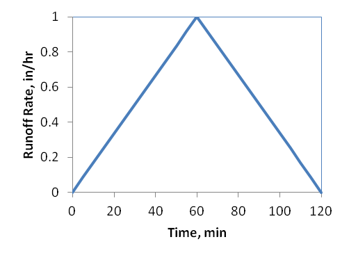
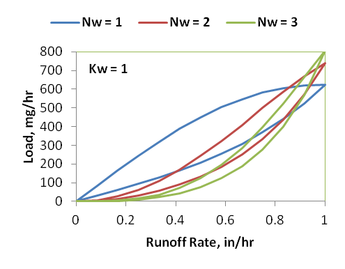
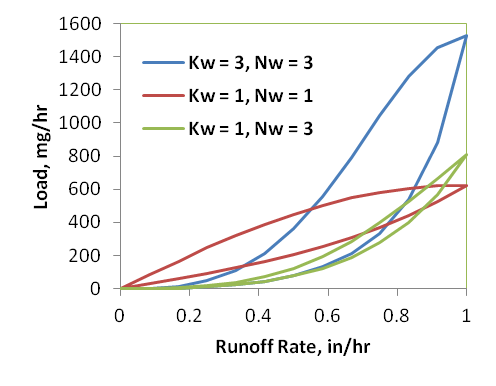
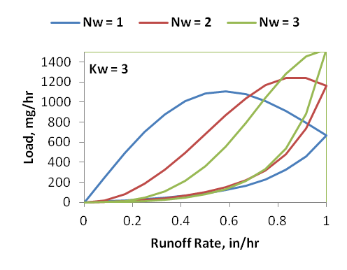
Figure 4‑4 Simulated load variations within a storm as a function of runoff rate
Procedures for calibrating SWMM's buildup and washoff parameters have been developed by Jewell et al. (1978), Alley (1981), and Baffaut and Delleur (1990). The challenge of calibrating the exponential washoff parameters to individual storm events is that different events will produce different parameter estimates. An example of this is the study made by Avellaneda et al. (2009). Estimating washoff parameters by minimizing the sum of squared differences between the observed and predicted suspended solids concentrations for each of 22 different storm events on a 7.4 acre parking lot resulted in a coefficient of variation (CV or standard deviation / mean) for *KW* of 1.8. (The CV for *NW* was only 0.2). Such variability presents problems in selecting a single set of values that will generate reliable pollutographs in future simulations.
Reproducing the time variation of washoff concentration within a storm event may be too lofty a goal to achieve given the simplified representation of the washoff process in SWMM. Instead, it might be more realistic to calibrate against the total mass of washoff produced over a number of storm events. This is the approach used by Behera et al. (2006) using a probabilistic model and by Tetra Tech (2010) using SWMM itself. In the latter case, the choice of parameter values was based on achieving a target annual pollutant loading (lbs/ac-yr) for each combination of pollutant and land use over a multi-year period of rainfall record. Table 4-3 shows the results achieved for the power buildup model and exponential washoff model for high-density residential land use.
Table 4‑3 Buildup/washoff calibration against annual loading rate for high-density residential land use Source: Tetra Tech (2010).
| Pollutant1 | Buildup | Washoff | Calibration Results (kg/ac/yr) | ||||||
|---|---|---|---|---|---|---|---|---|---|
| **Bmax** | **KB** | **NB** | **KW** | **NW** | Target | Calibrated | Error | ||
| TP | 4.75 | 0.031 | 0.42 | 0.71 | 1.37 | 0.45 | 0.449 | 0.2% | |
| TSS | 28.12 | 0.76 | 1.26 | 5.91 | 1.46 | 190.51 | 190.57 | 0% | |
| TN | 18.94 | 0.027 | 0.88 | 4.31 | 0.57 | 2.81 | 2.811 | 0.04% | |
| Zn | 4.78 | 0.013 | 0.088 | 7.22 | 1.11 | 0.32 | 0.322 | 0.6% |
1TP = total phosphorus, TSS = total suspended solids, TN = total nitrogen and Zn = zinc.
The exponential washoff model is most suitable when the pollutant load (mass/sec) versus runoff flow monitored during a storm event plot as a loop, as in Figure 4-4, since it tends to produce lower loads at the end of storm events as the buildup supply becomes depleted. The rating curve washoff model will work better when the load versus flow data plot as a straight line on log-log axes. On the basis of the previous discussion of rating curves based on sediment data, it is expected that the exponent, *NW*, would be in the range of 1.5 to 3.0 for constituents that behave like particulates. For dissolved constituents, the exponent will tend to be less than 1.0 since concentration often decreases as flow increases, and concentration is proportional to flow to the power *NW* - 1. (Constant concentration would use *NW* = 1.0.) Much more variability is expected for *KW*. The rating curve method is generally easiest to use when only total runoff volumes and pollutant loads are available for calibration. In this case a pure regression approach should suffice to determine parameters *KW* and *NW*.
As a part of the NPDES stormwater permitting program and as a result of many special studies, there are numerous sources of local event mean concentration (EMC) data available for stormwater. EMC values are usually measured by laboratory analysis of flow- and time-weighted composite samples. EMCs are often the only samples available, in order to save on laboratory costs that would be involved in measurements of several points along the storm hydrograph, although the latter, intra-event samples are particularly valuable data. As a practical matter, EMCs are the most common parameters used to estimate nonpoint water quality loads in SWMM and in most other models.
A primary source of EMC data is the Nationwide Urban Runoff Program (NURP), conducted by EPA in the early 1980s (US EPA, 1983). Sampling was conducted for 28 NURP projects which included 81 specific sites and more than 2,300 separate storm events. Table 2-3 presents a summary of the EMCs found from that study. The Center for Watershed Protection has put together a more comprehensive list of national EMCs that includes not just the NURP results but also additional data obtained from the U.S. Geological Survey (USGS), as well as stormwater monitoring conducted for EPA's National Pollutant Discharge Elimination System (NPDES) stormwater program. These are shown in Table 4-4.
When evaluating stormwater EMC data, it is important to keep in mind that regional EMCs can differ sharply from the reported national pollutant EMCs. Differences in EMCs between regions are often attributed to the variation in the amount and frequency of rainfall and snowmelt. Table 4-5 presents a breakdown of EMCs by different regions of the US classified by rainfall amounts.
Table 4‑4 National EMC's for stormwater Source: CWP (2003).
| Pollutant | Mean EMC | Median EMC | Number of Events Sampled |
|---|---|---|---|
| Sediment (mg/L) | |||
| TSS | 78.4 | 54.5 | 3047 |
| Organic Carbon (mg/L) | |||
| TOC | 17 | 15.2 | 19 studies |
| BOD | 14.1 | 11.5 | 1035 |
| COD | 52.8 | 44.7 | 2639 |
| MTBE | N/R | 1.6 | 592 |
| Nutrients (mg/L) | |||
| Total P | 0.32 | 0.26 | 3094 |
| Soluble P | 0.13 | 0.10 | 1091 |
| Total N | 2.39 | 2.00 | 2016 |
| Total Kjeldahl N | 1.73 | 1.47 | 2693 |
| Nitrite and Nitrate | 0.66 | 0.53 | 2016 |
| Metals (ug/L) | |||
| Copper | 13.4 | 11.1 | 1657 |
| Lead | 67.5 | 50.7 | 2713 |
| Zinc | 162 | 129 | 2234 |
| Cadmium | 0.7 | 0.5 | 150 |
| Chromium | 4.0 | 7.0 | 164 |
| Hydrocarbons (mg/L) | |||
| PAH | 3.5 | N/R | N/R |
| Oil & Grease | 3 | N/R | N/R |
| Bacteria and Pathogens (colonies/100 mL) | |||
| Fecal Coliform | 15,038 | N/R | 34 |
| Fecal Streptococci | 35,351 | N/R | 17 |
| Pesticides (ug/L) | |||
| Diazinon | N/R | 0.025 | 326 |
| Atrazine | N/R | 0.023 | 327 |
| Prometon | N/R | 0.031 | 327 |
| Simazine | N/R | 0.039 | 327 |
| Chloride (mg/L) | |||
| Chloride | N/R | 397 | 282 |
Table 4‑5 EMC's for different regions Source: CWP (2003)
(units are mg/L except for metals which are in ug/L)
| Pollutant / Metric | National | Phoenix, AZ | San Diego, CA | Boise, ID | Denver, CO | Dallas, TX | Marquette, MI | Austin, TX | MD | Louisville, KY | GA | FL | MN (Snow) |
|---|---|---|---|---|---|---|---|---|---|---|---|---|---|
| Annual Rainfall (in) | N/A | 7.1 | 10 | 11 | 15 | 28 | 32 | 32 | 41 | 43 | 51 | 52 | N/R |
| Number of Events | 3000 | 40 | 36 | 15 | 35 | 32 | 12 | N/R | 107 | 21 | 81 | N/R | 49 |
| TSS | 78.4 | 227 | 330 | 116 | 242 | 663 | 159 | 190 | 67 | 98 | 258 | 43 | 112 |
| Total N | 2.39 | 3.26 | 4.55 | 4.13 | 4.06 | 2.7 | 1.87 | 2.35 | N/R | 2.37 | 2.52 | 1.74 | 4.30 |
| Total P | 0.32 | 0.41 | 0.7 | 0.75 | 0.65 | 0.78 | 0.29 | 0.32 | 0.33 | 0.32 | 0.33 | 0.38 | 0.70 |
| Soluble P | 0.13 | 0.17 | 0.4 | 0.47 | N/R | N/R | 0.04 | 0.24 | N/R | 0.21 | 0.14 | 0.23 | 0.18 |
| Copper | 14 | 47 | 25 | 34 | 60 | 40 | 22 | 16 | 18 | 15 | 32 | 1.4 | N/R |
| Lead | 68 | 72 | 44 | 46 | 250 | 330 | 49 | 38 | 12.5 | 60 | 28 | 8.5 | 100 |
| Zinc | 162 | 204 | 180 | 342 | 350 | 540 | 111 | 190 | 143 | 190 | 148 | 55 | N/R |
| BOD | 14.1 | 109 | 21 | 89 | N/R | 112 | 15.4 | 14 | 14.4 | 88 | 14 | 11 | N/R |
| COD | 52.8 | 239 | 105 | 261 | 227 | 106 | 66 | 98 | N/R | 38 | 73 | 64 | 112 |
N/R: Not Recorded
 1.13.2