|
OpenSWMM Engine
6.0.0-alpha.4
Data-oriented, plugin-extensible SWMM Engine (6.0.0-alpha.4)
|
|
OpenSWMM Engine
6.0.0-alpha.4
Data-oriented, plugin-extensible SWMM Engine (6.0.0-alpha.4)
|
Low impact development (LID) controls are landscaping practices designed to capture and retain stormwater generated from impervious surfaces that would otherwise run off of a site. They are also referred to as green infrastructure (GI), integrated management practices (IMPs) sustainable urban drainage systems (SUDS), and stormwater control measures (SCMs). See Fletcher et al. (2015) for a review of this terminology. Prince Georges County (1999a) describes the LID concept and its application to stormwater management in more detail. Additional informational resources are available from the following US EPA web sites:
and from the Low Impact Development Center (http://lowimpactdevelopment.org).
SWMM 5 can explicitly model the following types of LID practices:
| LID Control Type | Description | Image |
|---|---|---|
| Bio-retention Cells | Depressions that contain vegetation grown in an engineered soil mixture placed above a gravel storage bed. They provide storage, infiltration and evaporation of both direct rainfall and runoff captured from surrounding areas. Street planters and bio-swales are common examples of bio-retention cells. |
|
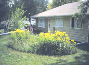
| Rain Gardens | A type of bio-retention cell consisting of just the engineered soil layer with no gravel bed below it. |
|
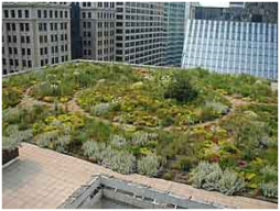
| Green Roofs | Another variation of a bio-retention cell that have a soil layer above a thin layer of synthetic drainage mat material or coarse aggregate that conveys excess water draining through the soil layer off of the roof. |
|
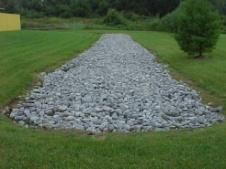
| Infiltration Trenches | Narrow ditches filled with gravel that intercept runoff from upslope impervious areas. They provide storage volume and additional time for captured runoff to infiltrate into the native soil below. |
|
| Continuous Permeable Pavement | Street or parking areas paved with a porous concrete or asphalt mix that sits above a gravel storage layer. Rainfall passes through the pavement into the storage layer where it can infiltrate into the site's native soil. |
|
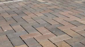
| Block Paver | Systems consist of impervious paver blocks placed on a sand or pea gravel bed with a gravel storage layer below. Rainfall is captured in the open spaces between the blocks and conveyed to the storage zone where it can infiltrate into the site's native soil. |
|
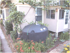
| Rain Barrels (or Cisterns) | Containers that collect roof runoff during storm events and can either release or re-use the rainwater during dry periods. |
|
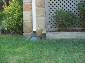
| Rooftop Disconnection | Has roof downspouts discharge to pervious landscaped areas and lawns instead of directly into storm drains. It can also model roofs with directly connected drains that overflow onto pervious areas. |
|
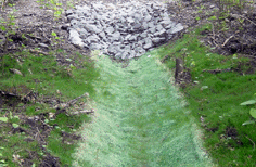
| Vegetative Swales | Channels or depressed areas with sloping sides covered with grass and other vegetation. They slow down the conveyance of collected runoff and allow it more time to infiltrate into the native soil. |
|
Bio-retention cells, infiltration trenches, and permeable pavement systems can contain optional underdrain systems in their gravel storage beds to convey excess captured runoff off of the site and prevent the unit from flooding. They can also have an impermeable floor or liner that prevents any infiltration into the native soil from occurring. Infiltration trenches and permeable pavement systems can also be subjected to a decrease in hydraulic conductivity over time due to clogging. Other LID practices, such as preservation of natural areas, reduction of impervious cover, and soil restoration, can be modeled by using SWMM's conventional runoff elements.
LID is a distributed method of runoff source control, that uses surface and landscape modifications located on or adjacent to impervious areas that generate most of the runoff in urbanized areas. For this reason SWMM considers LID controls to be part of its Subcatchment object, where each control is assigned a fraction of the subcatchment's impervious area whose runoff it captures. The design variables that affect the hydrologic performance of LID controls include the properties of the media (soil and gravel) contained within the unit, the vertical depth of its media layers, the hydraulic capacity of any underdrain system used, and the surface area of the unit itself. Although some LID practices can also provide significant pollutant reduction benefits (Hunt et al., 2006; Li and Davis, 2009), at this time SWMM only captures the reduction in runoff mass load resulting from the reduction in runoff flow volume.
Several different approaches have been used in the past to model LID hydrology. One simple scheme uses the void volume available in the LID unit (Davis and McCuen, 2005), possibly combined with a modified Curve Number for LID areas (Prince Georges County, 1999b), to determine what depth of storm event will be captured. Although useful for initial sizing, it ignores the effects that varying rainfall intensity and event frequency have on surface infiltration, soil moisture retention, and storage capacity. At the other end of the spectrum are detailed soil physics models, typically based on the Richards equation, that estimate the flows and moisture levels for a single LID unit over the course of a rainfall event (see Dussaillant et al., (2004) and He and Davis, (2011)). These approaches are too computationally intensive to be used in a general purpose engineering model like SWMM, where hundreds of LID units might be deployed throughout a large study area. A third approach, suggested by Huber et al. (2006) is to utilize SWMM's conventional elements and features, such as internal routing within subcatchments and multiple storage units connected by flow regulator links, to approximate the behavior of LID units. Unfortunately, an accurate representation of LID behavior can require a very complex arrangement of SWMM elements (see Zhang et al. (2006) and Lucas (2010) for examples). To circumvent these issues, SWMM 5 treats LID controls as an additional type of discrete element, using a unit process-based representation of their behavior (Rossman, 2010) that provides a reasonable level of accuracy for simulating dynamic rainfall events in a computationally efficient manner.
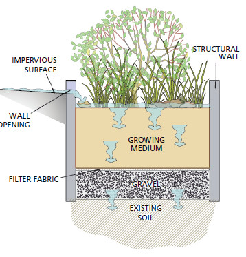
A typical bio-retention cell (see panel A of Figure 6-1) will serve as an example for developing a generic LID performance model. This generic model can then be customized as need be to describe the behavior of other types of LID controls.
Conceptually a bio-retention cell can be represented by a number of horizontal layers as shown in panel B of Figure 6-1. The surface layer (layer 1) receives both direct rainfall and runoff captured from other areas. It loses water through infiltration into the soil layer below it, by evapotranspiration (ET) of any ponded surface water, and by any surface runoff that might occur. The soil layer (layer 2) contains an engineered soil mix that can support vegetative growth. It receives infiltration from the surface layer and loses water through ET and by percolation into the storage layer below it. The storage layer (layer 3) consists of coarse crushed stone or gravel. It receives percolation from the soil zone above it and loses water by infiltration into the underlying natural soil and by outflow through a perforated pipe underdrain system if present.
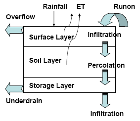
**(A)** **(B)**
Figure 6‑1 A typical bio-retention cell
To model the hydrologic performance of this LID unit the following simplifying assumptions are made:
Under these assumptions the LID unit can be modeled by solving a set of simple flow continuity equations. Each equation describes the change in water content in a particular layer over time as the difference between the inflow and the outflow water flux rates that the layer sees, expressed as volume per unit area per unit time. These equations can be written as follows:
Surface Layer
\[\phi_{1}\frac{\partial d_{1}}{\partial t} = i + q_{0} - e_{1} - f_{1} - q_{1}\]
(6-1)
Soil Layer
\[D_{2}\frac{\partial\theta_{2}}{\partial t} = f_{1} - e_{2} - f_{2}\]
(6-2)
Storage Layer
\[\phi_{3}\frac{\partial d_{3}}{\partial t} = f_{2} - {e_{3} - f}_{3} - q_{3}\]
(6-3)
where:
*d1* = depth of water stored on the surface (ft),
*θ2* = soil layer moisture content (volume of water / total volume of soil),
*d3* = depth of water in the storage layer (ft),
i = precipitation rate falling directly on the surface layer (ft/sec),
*q0* = inflow to the surface layer from runoff captured from other areas (ft/sec),
*q1* = surface layer runoff or overflow rate (ft/sec),
*q3* = storage layer underdrain outflow rate (ft/sec),
*e1* = surface ET rate (ft/sec),
*e2* = soil layer ET rate (ft/sec),
*e3* = storage layer ET rate (ft/sec),
*f1* = infiltration rate of surface water into the soil layer (ft/sec),
*f2* = percolation rate of water through the soil layer into the storage layer (ft/sec),
*f3* = exfiltration rate of water from the storage layer into native soil (ft/sec),
\(\phi_{1}\) = void fraction of any surface volume (i.e., the fraction of freeboard above the surface not filled with vegetation)
\(\phi_{2}\) = porosity (void volume / total volume) of the soil layer (used later on),
\(\phi_{3}\) = void fraction of the storage layer (void volume / total volume),
*D1* = freeboard height for surface ponding (ft) (used later on),
*D2* = thickness of the soil layer (ft),
*D3* = thickness of the storage layer (ft) (used later on).
The flux terms (q, e, and f) in these equations are functions of the current water content in the various layers (*d1, θ2,* and *d3*) and specific site and soil characteristics. This set of coupled equations can be solved numerically at each runoff time step to determine how an inflow hydrograph to the LID unit (*i + q0*) is converted into hydrographs for surface runoff (*q1*), underdrain outflow (*q3*), and exfiltration into the surrounding native soil (*f3*). As applied to a bio-retention cell, this generic model is similar in spirit to the RECARGA model developed at the University of Wisconsin – Madison (Atchison and Severson, 2004) for rain gardens with no gravel storage zone. How each of the flux terms in Equations 6-1 to 6-3 is computed will now be discussed.
Surface Inflow (*i + q0*)
Inflow to the surface layer comes from both direct rainfall (i) and runoff from impervious areas captured by the bio-retention cell (*q0*). Within each runoff time step these values are provided by SWMM's runoff computation as described in Chapter 3 of Volume I of this manual.
Surface Infiltration (*f1*)
The infiltration of surface water into the soil layer, *f1*, can be modeled with the Green-Ampt equation:
\[f_{1} = K_{2S}\left( 1 + \frac{\left( \phi_{2} - \theta_{20} \right)(d_{1} + \psi_{2})}{F} \right)\]
(6-4)
where
*f1* = infiltration rate (ft/sec), *K2S* = soil's saturated hydraulic conductivity (ft/sec)
*θ20* = moisture content at the top of the soil layer (fraction),
*ψ2* = suction head at the infiltration wetting front formed in the soil (ft)
F = cumulative infiltration volume per unit area over a storm event (ft)
This equation applies only after a saturated condition develops at the top of the soil zone. Prior to this all inflow (*i + q0*) infiltrates. The initial value of *θ20* for a dry soil would be its residual moisture content or its wilting point. It increases after each rainfall event, then decreases during dry periods. The details of implementing the Green-Ampt model over successive time steps are described in Chapter 4 of Volume I of this manual. The properties *K2S*, *φ2*, and *ψ2* for the bio-retention cell's amended soil can be different from those of the site's natural soil. This can produce a different infiltration rate into the LID unit when compared to that for rest of the subcatchment.
Evapotranspiration (e)
Evapotranspiration (ET) of water stored within the bio-retention cell is computed from the same user-supplied time series of daily potential ET rates that are used in SWMM's runoff module (see Chapter 2 of Volume I). The calculation proceeds from the surface layer downwards, where any un-used potential ET is made available to the next lower layer. So at any time t:
\[e_{1} = min\left\lbrack E_{0}(t),\ \frac{d_{1}}{\Delta t} \right\rbrack\]
(6-5)
\[e_{2} = min\left\lbrack E_{0}(t) - e_{1}\ ,\frac{\left( \theta_{2} - \theta_{WP} \right)D_{2}}{\mathrm{\Delta}t} \right\rbrack\]
(6-6)
\[e_{3} = \left\{ \begin{aligned} (6-7) \min\left\lbrack E_{0}(t) - e_{1} - e_{2}\ ,\ \frac{\phi_{3}d_{3}}{\mathrm{\Delta}t} \right\rbrack,\ \ \ & \theta_{2} < \phi_{2} \\ 0,\ \ & \theta_{2} \geq \phi_{2} \end{aligned} \right.\ \]
where \(E_{0}(t)\) is the potential ET rate that applies for time t, ∆t is the time step used to numerically evaluate the governing flow balance equations 6-1 to 6-3, and \(\theta_{WP}\) is the user-supplied wilting point soil moisture content. A soil's wilting point is the moisture content below which plants can no longer extract water from the soil. Thus when the soil moisture *θ2* reaches the wilting point there is no contribution to ET from the soil layer.
Note how ET from each layer is limited by the amount of potential ET remaining and the amount of water stored in the layer. In addition:
Soil Percolation (*f2*)
The rate of percolation of water through the soil layer into the storage layer below it (*f2)* can be modeled using Darcy's Law in the same manner used in SWMM's existing groundwater module (see Chapter 5 of Volume I). The resulting equation for this flux is:
\[f_{2} = \left\{ \begin{aligned} (6-8) K_{2S}\exp\left( - HCO\left( \phi_{2} - \theta_{2} \right) \right),\ \ \ & \theta_{2} > \theta_{FC} \\ 0,\ \ & \theta_{2} \leq \theta_{FC} \end{aligned} \right.\ \]
where *K2S* is the soil's saturated hydraulic conductivity (ft/sec), HCO is a decay constant derived from moisture retention curve data that describes how conductivity decreases with decreasing moisture content, and *θFC* is the soil's field capacity moisture content. The same expression for unsaturated soil percolation is used in SWMM's groundwater module. When the moisture content *θ2* drops below the field capacity moisture level *θFC* then the percolation rate becomes zero. This limit is in accordance with the concept of field capacity as the drainable soil water that cannot be removed by gravity alone (Hillel, 1982, p. 243).
Bottom Exfiltration (*f3*)
The exfiltration rate from the bottom of the storage zone into native soil would normally depend on the depth of stored water and the moisture profile of the soil beneath the LID unit. Since the latter is not known, SWMM assumes that the exfiltration rate \(f_{3}\) is simply the user-supplied saturated hydraulic conductivity of the native soil beneath the LID unit, *K3S*. Setting *K~3S\ ~*to zero indicates that the bio-retention cell has an impermeable bottom.
Underdrain Flow (*q3*)
Because the hydraulics of perforated pipe underdrains can be complicated (see van Schilfgaarde 1974) SWMM uses a simple empirical power law to model underdrain outflow *q3*:
\[q_{3} = C_{3D}\left( h_{3} \right)^{\eta_{3D}}\]
(6-9)
where
*h3* = hydraulic head seen by underdrain, (ft) *C3D* = underdrain discharge coefficient ( \(\frac{{ft}^{- (\eta_{3D} - 1)}}{\sec}\))
*η3D* = underdrain discharge exponent
The hydraulic head *h3* seen by the underdrain varies with the height of water above it in the following fashion:
\[h_{3} = 0\]
for \(d_{3} \leq D_{3D}\)
\[h_{3} = d_{3} - D_{3D}\]
for \(D_{3D} < d_{3} < D_{3}\)
\[h_{3} = \left( D_{3} - D_{3D} \right) + \frac{\left( \theta_{2} - \theta_{FC} \right)}{\left( \phi_{2} - \theta_{FC} \right)D_{2}}\]
for \(d_{3} = D_{3}\) and \(\theta_{FC} < \theta_{2} < \phi_{2}\)
\[h_{3} = \left( D_{3} - D_{3D} \right) + D_{2} + d_{1}\]
for \(d_{3} = D_{3}\) and \(\theta_{2} = \phi_{2}\)
where *D3D* is the height of drain opening above bottom of storage layer (ft) and \(\theta_{FC}\) is the soil layer's field capacity moisture content below which water does not drain freely from the soil.
Underdrains introduce three additional parameters *C3D, η3D,* and *D3D*, into the description of a bio-retention cell. There is no underdrain flow until the depth of water in the storage layer reaches the drain offset height. Choosing a value of 0.5 for *η3D* makes the drain flow formula equivalent to the standard orifice equation, where *C3D* incorporates both the normal orifice discharge coefficient and available flow area. Setting *C3D* to zero indicates that no underdrain is present. The flow rate computed with Equation 6-9 should be considered a maximum potential value. The actual underdrain flow at any time step will be the smaller of this value and the amount of water available to the underdrain.
Surface Runoff (*q1*)
It is assumed that any ponded surface water in excess of the maximum freeboard (or depression storage) height *D1* becomes immediate overflow. Therefore:
\[q_{1} = max\left\lbrack \frac{\left( d_{1} - D_{1} \right)}{\mathrm{\Delta}t},\ 0 \right\rbrack\]
(6-10)
Flux Limits
Limits must be imposed on the various bio-retention cell flux rates to insure that at any given time step the moisture levels in the soil and storage layers do not go negative nor exceed the layer's capacity. These limits are evaluated in the order listed below.
The soil percolation rate *f2* is limited by the amount of drainable water currently in the soil layer plus the net amount of water added to it over the time step:
\[f_{2} = min\left\lbrack \frac{f_{2}\ ,\left( \theta_{2} - \theta_{FC} \right)D_{2}}{\mathrm{\Delta}t} + f_{1} - e_{2} \right\rbrack\]
(6-11)
The storage exfiltration rate *f3* is limited by the amount of water currently in the storage layer plus the net amount of water added to it over the time step:
\[f_{3} = min\left\lbrack \frac{f_{3}\ ,d_{3}\phi_{3}}{\mathrm{\Delta}t} + f_{2} - e_{3} \right\rbrack\]
(6-12)
When an underdrain is used, the drain flow *q3* is limited by the amount of water stored above the drain offset plus any excess inflow from the soil layer that remains after storage exfiltration is accounted for:
\[q_{3} = min\left\lbrack \frac{q_{3}\ ,{\left( d_{3} - D_{3D} \right)\phi}_{3}}{\mathrm{\Delta}t} + f_{2} - f_{3} - e_{3} \right\rbrack\]
(6-13)
The soil percolation rate is also limited by the amount of unused volume in the storage layer plus the net amount of water removed from storage over the time step.
\[f_{2} = min\left\lbrack \frac{f_{2}\ ,{\left( D_{3} - d_{3} \right)\phi}_{3}}{\mathrm{\Delta}t} + f_{3} + q_{3} + e_{3} \right\rbrack\]
(6-14)
The rate *f1* at which water can infiltrate into the soil layer is limited by the amount of empty pore space available plus the volume removed by drainage and evaporation over the time step.
\[f_{1} = min\left\lbrack \frac{f_{1}\ ,{\left( \phi_{2} - \theta_{2} \right)D}_{2}}{\mathrm{\Delta}t} + f_{2} + e_{2} \right\rbrack\]
(6-15)
When the unit becomes completely saturated (i.e., *θ2 = φ2* and *d3 = D3*) then the vertical flux of water through both the soil and storage layers has to be the same since there is a common fully wetted interface between them. For this special case, if \(f_{2} > f_{3} + q_{3}\) then \(f_{2} = f_{3} + q_{3}\). Otherwise \(f_{3} = min\left\lbrack f_{3}\ ,f_{2} \right\rbrack\) and \(q_{3} = max\left\lbrack f_{3} - f_{2}\ ,0 \right\rbrack.\) In addition the surface infiltration rate *f1* cannot exceed the adjusted soil percolation rate: \(f_{1} = min\left\lbrack f_{1},f_{2} \right\rbrack\). (Note that because the unit is saturated no sub-surface ET occurs and therefore does not influence these limits.)
It is worth noting that this simple representation of a bio-retention cell uses a total of 15 user-supplied parameters in its description: two surface layer parameters (*φ1, D1*) seven soil layer parameters (*φ2, θFC, θWP, K2S, ψ2, HCO, D2*), three storage layer parameters *(φ3, K3S*, *D3)* and three underdrain parameters (*C3D, η3D*, *D3D*). The six constants that define the soil layer's moisture limits ( \(\phi_{2},\ {\psi_{2},\ \theta}_{FC},\ \theta_{WP}\)) and hydraulic conductivity ( \(K_{2S},\ HCO\)) are the same parameters used for infiltration and groundwater flow in SWMM's hydrology module (see Chapters 4 and 5 of Volume I). Because the soil used in a bio-retention cell is an engineered mix chosen to provide good drainage and support plant growth its properties will likely be different than those of the site's native soil. Recommended values for the various parameters associated with all types of LID controls will be presented later on in Section 6.6.
The governing flow balance equations for the other LID controls modeled by SWMM are similar in form to those for bio-retention cells. The following sub-sections discuss the models for rain gardens, green roofs, infiltration trenches, permeable pavement, rain barrels, rooftop disconnection, and vegetative swales in that order.
SWMM defines a rain garden as a bio-retention cell without a storage layer. Its governing equations are therefore:
Surface Layer
\[\phi_{1}\frac{\partial d_{1}}{\partial t} = i + q_{0} - e_{1} - f_{1} - q_{1}\]
(6-16)
Soil Layer
\[D_{2}\frac{\partial\theta_{2}}{\partial t} = f_{1} - e_{2} - f_{2}\]
(6-17)
The nominal soil percolation rate *f2* is computed via Equation 6-8. It is then limited to the smaller of this value, the amount of drainable water available in the soil layer (Equation 6-11) and the saturated hydraulic conductivity of the native soil beneath the rain garden (*K3S*). The remaining flux rates are computed as described earlier.
SWMM's green roof is also similar to a bio-retention cell, except it uses a drainage mat instead of gravel aggregate in its storage layer. Drainage mats are thin, multi-layer fabric mats with ribbed undersides that convey water. They have somewhat limited water storage and drainage capacity and are therefore mostly used on sloped roofs. Another type of roof drainage system also suitable for flatter roofs uses slotted pipes placed in a gravel bed and is therefore functionally equivalent to a bio-retention cell with an impermeable bottom ( \(K_{3S} = 0\)) and an underdrain.
The governing equations for a green roof with a drainage mat would be:
Surface Layer
\[\phi_{1}\frac{\partial d_{1}}{\partial t} = i - e_{1} - f_{1} - q_{1}\]
(6-18)
Soil Layer
\[D_{2}\frac{\partial\theta_{2}}{\partial t} = f_{1} - e_{2} - f_{2}\]
(6-19)
Drainage Mat Layer
\[\phi_{3}\frac{\partial d_{3}}{\partial t} = f_{2} - e_{3} - q_{3}\]
(6-20)
Note the absence of the captured runoff term *q0* in Equation 6-18 since a green roof would only be capturing direct rainfall. There is also no exfiltration term *f3* since the bottom of a green roof consists of an impermeable membrane.
The runoff rate from the soil layer surface (*q1*) is computed using the Manning equation for uniform overland flow. Under the assumption that the width of the flow area is much greater than the depth of flow the Manning equation becomes:
\[q_{1} = \frac{1.49}{n_{1}}\sqrt{S_{1}}(\frac{W_{1}}{A_{1})\phi_{1}\left( d_{1} - D_{1} \right)^{\frac{5}{3}}}\]
(6-21)
where
*n1* = surface roughness coefficient,
*S1* = surface slope (ft/ft),
*W1* = total length along edge of the roof where runoff is collected (ft),
*D1* = surface depression storage depth (ft),
*A1* = roof surface area (ft2).
All of these surface parameters are supplied by the user as part of the green roof's design. The "surface" that these parameters describe is the surface of the soil layer. The \(\frac{W_{1}}{A_{1}}\) term represents the length of the flow path that excess water takes before it enters the roof's drain system (see Figure 6-2). When the depth of ponded water *d1* is at or below the depression storage depth *D1* then no surface outflow occurs.
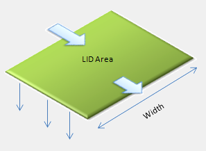
Figure 6‑2 Flow path across the surface of a green roof
Another option for surface outflow is to have any ponded surface water in excess of the depression storage *D1* become instantaneous runoff using Equation 6-10. This is done by setting either *n1*, *S1*, or *W1* to zero. This may be a better choice for roofs with short flow path lengths or flat roofs that use internal roof drains.
The drainage mat flow rate *q3*in Equation 6-20 is assumed to obey uniform open channel flow within the channels of the mat. Thus it can be expressed as:
\[q_{3} = \frac{1.49}{n_{3}}\sqrt{S_{1}}(\frac{W_{1}}{A_{1}){\phi_{3}\left( d_{3} \right)}^{\frac{5}{3}}}\]
(6-22)
where *n3* is a roughness coefficient for the mat and *S1*, *W1*, and *A1* are the same slope, outflow face width, and roof surface area, respectively, used to evaluate surface overflow (*q1*).
The remaining flux rates in Equations 6-18 to 6-20 are evaluated in the same fashion as for the bio-retention cell. In addition, the same flux limiting conditions for the bio-retention cell (Equations 6-11 through 6-15) are applied to the green roof to insure that the values used for *f1*, *f2*, and *q3* maintain feasible moisture levels for the soil and drainage layers after each time step.
An infiltration trench can be represented in the same fashion as a bio-retention cell but having just a surface and a storage layer. The governing equations are:
Surface Layer
\[\frac{\partial d_{1}}{\partial t} = i + q_{0} - e_{1} - f_{1} - q_{1}\]
(6-23)
Storage Layer
\[\phi_{3}\frac{\partial d_{3}}{\partial t} = f_{1} - {e_{3} - f}_{3} - q_{3}\]
(6-24)
where now *f1* is the trench's external inflow plus any ponded surface water that drains into the storage layer over the time step:
\[f_{1} = i + \ q_{0} + \frac{d_{1}}{\mathrm{\Delta}t}\]
(6-25)
Nominal values for the remaining flux terms are evaluated in the same fashion as for the bio-retention cell. The surface void fraction *φ1* does not appear in the surface layer equation since a gravel-filled trench would have no vegetative growth above it.
These nominal rates are subject to the following constraints:
The storage exfiltration rate *f3* is limited by the amount of water currently in the storage layer plus the net amount of water added to it over the time step:
\[f_{3} = min\left\lbrack \frac{f_{3}\ ,d_{3}\phi_{3}}{\mathrm{\Delta}t} + f_{1} - e_{3} \right\rbrack\]
(6-26)
When an underdrain is used, the drain flow *q3* is limited by the amount of water stored above the drain offset plus any excess inflow from the surface that remains after storage exfiltration is accounted for:
\[q_{3} = min\left\lbrack \frac{q_{3}\ ,{\left( d_{3} - D_{3D} \right)\phi}_{3}}{\mathrm{\Delta}t} + f_{1} - f_{3} - e_{3} \right\rbrack\]
(6-27)
The surface inflow rate *f1* is limited by the amount of empty storage layer space available plus the volume removed by exfiltration, underdrain flow, and evaporation over the time step:
\[f_{1} = min\left\lbrack \frac{f_{1}\ ,\left( D_{3} - d_{3} \right)\phi_{3}}{\mathrm{\Delta}t} + f_{3} + q_{3} + e_{3} \right\rbrack\]
(6-28)
Figure 6-3 illustrates a typical continuous permeable pavement system. It consists of a pervious concrete or asphalt top layer, an optional sand filter or bedding layer beneath that and a gravel storage layer on the bottom which can contain an optional slotted pipe underdrain system. It introduces a new type of layer, a pavement layer (layer 4), which is characterized by its thickness (*D4*), porosity (*φ4*), and permeability *K4*. A block paver system would look the same but with an additional parameter (*F4*) representing the fraction of the surface area taken up by the impermeable paver blocks and where the porosity and permeability refer to the fine gravel used to fill the seams between blocks. For continuous systems *F4* would be 0.
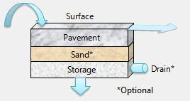
Figure 6‑3 Representation of a permeable pavement system
The governing equations for permeable pavement with a sand layer included are:
Surface Layer
\[\frac{\partial d_{1}}{\partial t} = i + q_{0} - e_{1} - f_{1} - q_{1}\]
(6-29)
Pavement Layer
\[D_{4}\left( 1 - F_{4} \right)\frac{\partial\theta_{4}}{\partial t} = f_{1} - e_{4} - f_{4}\]
(6-30)
Sand Layer
\[D_{2}\frac{\partial\theta_{2}}{\partial t} = f_{4} - e_{2} - f_{2}\]
(6-31)
Storage Layer
\[\phi_{3}\frac{\partial d_{3}}{\partial t} = f_{2} - {e_{3} - f}_{3} - q_{3}\]
(6-32)
where \(\theta_{4}\) is the moisture content of the permeable pavement layer, \(f_{4}\) is the rate at which water drains out of the pavement layer, and all other terms have been defined previously. Note that when no sand layer is present, Equation 6-31 is removed and \(f_{4}\) replaces \(f_{2}\) in the storage layer Equation 6-32. Also, the surface void fraction *φ1* does not appear in the surface layer equation since a paved surface would have no vegetative growth above it.
The flux terms in these equations are evaluated in the same manner as for the bio-retention cell with the following exceptions:
Evaporation of any water stored in the pavement layer, *e4*, would proceed at the rate:
\[e_{4} = min\left\lbrack E_{0}(t) - e_{1}\ ,\frac{\theta_{4}D_{4}\left( 1 - F_{4} \right)}{\mathrm{\Delta}t} \right\rbrack\]
(6-33)
with *E0(t)* subsequently reduced by *e4* when ET from the layers below it is evaluated.
The nominal flux rate from the surface layer into the pavement layer (*f1*) is the same as for an infiltration trench:
\[f_{1} = i + \ q_{0} + \frac{d_{1}}{\mathrm{\Delta}t}\]
(6-34)
When evaluating underdrain outflow *q3*, once both the storage layer and sand layer (if present) become saturated, the head on the underdrain becomes:
\[h_{3} = \left( D_{3} - D_{3D} \right) + D_{2} + \frac{\theta_{4}D_{4}}{\phi_{4}}\]
(6-35)
The following adjustments are applied to the nominal flux rates in the order listed so that feasible moisture levels are maintained:
Pavement flux rate *f4* :
\[f_{4} = min\left\lbrack \frac{f_{4}\ ,\theta_{4}D_{4}}{\mathrm{\Delta}t} + f_{1} - e_{4} \right\rbrack\]
(6-36)
Soil percolation rate *f2* :
\[f_{2} = min\left\lbrack \frac{f_{2}\ ,\left( \theta_{2} - \theta_{FC} \right)D_{2}}{\mathrm{\Delta}t} + f_{4} - e_{4} \right\rbrack\]
(6-37)
Storage exfiltration rate *f3* :
\[f_{3} = min\left\lbrack \frac{f_{3}\ ,d_{3}\phi_{3}}{\mathrm{\Delta}t} + f_{2} - e_{3} \right\rbrack\]
(6-38)
where *f2 = f4* if there is no soil layer.
Underdrain flow *q3* (when present):
\[q_{3} = min\left\lbrack \frac{q_{3}\ ,{\left( d_{3} - D_{3D} \right)\phi}_{3}}{\mathrm{\Delta}t} + f_{2} - f_{3} - e_{3} \right\rbrack\]
(6-39)
where again *f2 = f4* if there is no soil layer.
with soil layer
\[\frac{f_{4} = min\lbrack f_{4}\ ,\left( \phi_{2} - \theta_{2} \right)D_{2}}{\mathrm{\Delta}t + f_{2} + e_{2}\rbrack}\]
(6-40)
without soil layer
\[\frac{f_{4} = min\lbrack f_{4}\ ,\left( D_{3} - d_{3} \right)\phi_{3}}{\mathrm{\Delta}t + e_{3} + f_{3} + q_{3}\rbrack}\]
(6-41)
Soil percolation rate *f2* :
\[f_{2} = min\left\lbrack \frac{f_{2}\ ,{\left( D_{3} - d_{3} \right)\phi}_{3}}{\mathrm{\Delta}t} + f_{3} + q_{3} + e_{3} \right\rbrack\]
(6-42)
Pavement inflow rate *f1* :
\[f_{1} = min\left\lbrack f_{1}\ ,\ \frac{\left( \phi_{4} - \theta_{4} \right)D_{4}\left( 1 - F_{4} \right)}{\mathrm{\Delta}t} + f_{4} + e_{4} \right\rbrack\]
(6-43)
The flux adjustments for fully saturated storage and sand layers follow those used for a bio-retention cell. When all of the sub-surface layers become saturated *(θ2* = *φ2*, *d3 = D3* and *θ4 = φ4*), and the unit is still receiving rainfall/runon then all flux rates are set equal to the limiting rate. The latter is the smaller of *f1, f4, f2* (if a sand layer is present), and *f3 + q3*. If the storage layer does not contain the limiting flux f*, then its outflow streams are adjusted as follows: \(q_{3} = min\left\lbrack q_{3}\ ,f^{*} \right\rbrack\) and \(f_{3} = f^{*} - q_{3}\).
A rain barrel can be modeled as just a storage layer that is all void space with a drain valve placed above an impermeable bottom. Only a single continuity equation is required:
Storage Layer
\[\frac{\partial d_{3}}{\partial t} = f_{1} - q_{1} - q_{3}\]
(6-44)
where *f1* now represents the amount of surface inflow captured by the barrel. Because the barrel is assumed to be covered there is no precipitation input and no evaporation flux. The general underdrain equation 6-7 would still be used to compute the barrel's drain flow *q3*. If the standard orifice equation is used to compute the drain outflow, then *η3D* in Equation 6-7 would be 0.5 and *C3D* would be:
\[C_{3D} = 0.6\left( \frac{A_{3}}{A_{1}} \right)\sqrt{2g}\]
(6-45)
where *A1* is the surface area of the barrel, *A3* is the area of the drain valve opening (ft2) and g is the acceleration of gravity (i.e., 32.2 ft/sec2). The outflow over a time step ∆t would be limited by the volume of water stored in the barrel:
\[q_{3} = min\left\lbrack q_{3}\ ,\frac{d_{3}}{\mathrm{\Delta}t} \right\rbrack\]
(6-46)
SWMM allows the drain valve to be closed prior to a rainfall event and then opened at some stipulated number of hours after rainfall ceases. If the valve is closed then *q3* would be 0.
The inflow to the barrel is the smaller of the external runoff *q0* applied to the barrel and the amount of empty storage available over the time step:
\[f_{1} = min\left\lbrack q_{0}\ ,\frac{\left( D_{3} - d_{3} \right)}{\mathrm{\Delta}t + q_{3}} \right\rbrack\]
(6-47)
And finally the barrel overflows at a rate *q1* when the runoff applied to the barrel exceeds its capacity to accept that amount of inflow:
\[q_{1} = max\left\lbrack 0\ ,q_{0} - f_{1} \right\rbrack\]
(6-48)
Rooftop areas contained within a SWMM subcatchment are normally treated as impervious surfaces whose runoff is directly connected to the subcatchment's storm drain outlet. By using SWMM's overland flow re-routing option it is possible to disconnect the rooftop area and make its runoff flow over the subcatchment's pervious area where it has the opportunity to infiltrate into the soil (see Section 3.6 of Volume I). The rooftop disconnection LID control provides another alternative to model rooftop runoff that allows for a higher level of detail than overland flow re-routing.
Figure 6-4 shows the physical configuration modeled by rooftop disconnection. Runoff from the roof surface is collected in a drain system of gutters, downspouts, and leaders. Any flow that exceeds the capacity of the roof drain system becomes overflow that can be re-routed onto pervious area. The roof drain flow can also be routed back onto pervious area (to disconnect the roof) or be sent to a storm sewer to keep the roof directly connected. Another option, used when modeling dual drainage systems (both street flow and sewer flow), is to allow the overflow to contribute to the major (street) system and the roof drain flow to the minor (sewer) system.
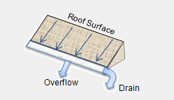
Figure 6‑4 Representation of rooftop disconnection
To model a rooftop in the same fashion as the other LID controls requires a single flow continuity equation for the roof surface:
Surface Layer
\[\frac{\partial d_{1}}{\partial t} = i - e_{1} - q_{1} - q_{3}\]
(6-49)
where now *q3* is interpreted as the flow rate per unit of roof area through the roof drain system and *q1* is the overflow rate from that system.
Evaporation from the roof surface (*e1*) is computed in the same fashion as for the surface of a bio-retention cell (Equation 6-4). The nominal runoff *q1* from the roof's surface, prior to entering the roof gutter, is also computed the same as for a green roof. The Manning equation 6-21 is used if information is provided on the roof's width, slope, and surface roughness. However now the roughness is for the roof surface itself and not the growth media found on a green roof. Otherwise Equation 6-10 is used to convert all flow in excess of any rooftop depression storage (*D1*) into immediate runoff. The amount of flow through the roof drain, *q3*, is the smaller of the nominal *q1* and the flow capacity of the roof drain system (*q3max*):
\[q_{3} = min\left\lbrack q_{1}\ ,q_{3max} \right\rbrack\]
(6-50)
Note that *q3max* is a user-supplied parameter with units of cfs per square foot of roof area. The actual overflow rate *q1* is simply the difference between its nominal rate and *q3*.
As shown in Figure 6-5, SWMM considers a vegetative swale to be a natural grass-lined trapezoidal channel that conveys captured runoff to another location while allowing it to infiltrate into the soil beneath it. It can be modeled with a single surface layer whose continuity equation is:
Surface Layer
\[A_{1}\frac{\partial d_{1}}{\partial t} = \left( i + q_{0} \right)A - (e_{1} + f_{1})A_{1} - q_{1}A\]
(6-51)
where *A1* is the surface area at water depth *d1* and A is the user-supplied surface area occupied by the swale across its full height *D1*. Unlike the other LID controls that were assumed to have a constant surface area throughout all layers, this equation accounts for a varying surface area as the depth of water in the swale changes.
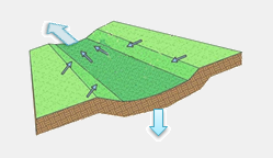
Figure 6‑5 Representation of a vegetative swale
From simple geometry, the relation between surface area *A1* and depth of flow *d1* is:
\[A_{1} = \frac{A}{W_{1}}\left\lbrack W_{1} - 2S_{X}\left( D_{1} - d_{1} \right) \right\rbrack\]
(6-52)
where *W1* is the width of the swale at its full height *D1* and *SX* is the slope (run over rise) of its trapezoidal side walls. The volume of water contained in the swale, *V1*, is the longitudinal length of the swale, \(\frac{A}{W_{1}}\), multiplied by the area of the wetted cross-section, *AX*:
\[V_{1} = \left( \frac{A}{W_{1}} \right)A_{X}\]
(6-53)
The wetted cross-sectional area is:
\[A_{X} = d_{1}\left( W_{X} + d_{1}S_{X} \right)\phi_{1}\]
(6-54)
where *WX* is the width across the bottom of the swale's cross section (equal to \(W_{1} - 2S_{X}D_{1}\)) and *φ1* is the fraction of the volume above the surface not occupied by vegetation.
The volumetric rate of evaporation of surface water in the swale, \(e_{1}A_{1}\), is the smaller of the external potential ET rate, \(E_{0}(t)A_{1}\) and the available volume of surface water over the time step, \(\frac{V_{1}}{\mathrm{\Delta}t}\). Because the swale is assumed to sit on top of the subcatchment's native soil, the infiltration rate *f1* is the same value computed for the pervious area of the subcatchment by SWMM's runoff module (see Chapter 4 of Volume I for details).
The swale's volumetric outflow rate, *q1A*, is computed using the Manning equation:
\[q_{1}A = \frac{1.49}{n_{1}}\sqrt{S_{1}}\ A_{X}\ R_{X}^{\frac{2}{3}}\]
(6-55)
where *n1* is the roughness of the swale's surface, *S1* is its slope in the direction of flow, and *RX* is its hydraulic radius (ft). The latter quantity is given by:
\[R_{X} = \frac{A_{X}}{\left( W_{X} + 2d_{1}\sqrt{1 + S_{X}^{2}} \right)}\]
(6-56)
To summarize, the parameters required to model a vegetative swale include its total surface area A, its top width *W1*, its maximum depth *D1*, its surface roughness *n1*, its longitudinal slope *S1, the slope of its side walls *S~x~, and fraction of its volume not occupied by vegetation *φ1*.
Clogging from fine sediment deposited within permeable pavement systems degrades infiltration rates over time (Ferguson, 2005) and their surfaces must be periodically vacuumed to maintain their performance (PWD, 2014). Infiltration trenches are also susceptible to clogging (US EPA, 1999) and typically require pretreatment with other BMPs, such as vegetated buffer strips, to remove coarse sediments (MDE, 2009).
SWMM uses a simplified approach to determine how clogging will reduce the hydraulic conductivity of permeable pavement and of the soil underneath a gravel storage layer over time. It is based on the empirically derived model proposed by Siriwardene et al. (2007) and its linearized form used by Lee et al. (2015). In those models the hydraulic conductivity of the media in question decreases over time as a continuous function of the cumulative sediment mass load passing through it. Because clogging is a long-term phenomenon, cumulative sediment mass load can be replaced by cumulative inflow volume by assuming a constant long-term average sediment inflow concentration. This inflow volume can be adjusted for the amount of void space in the relevant LID layer so that hydraulic conductivity reduction becomes a function of the number of the layer's void volumes processed by the LID unit.
If one defines a clogging factor CF as the number of layer void volumes treated to completely clog the layer and assumes a linear loss of conductivity with number of void volumes treated, then the conductivity K at some time t can be estimated as:
\[K(t) = K(0)\left( 1 - \frac{Q(t)V_{void}}{CF} \right)\]
(6-57)
where K(0) is the initial conductivity, V~void~ is the volume of void space per unit area in the LID layer, and Q(t) is the cumulative inflow volume (per unit area) to the LID unit up through time t. The latter quantity can be evaluated as:
\[Q(t) = \int_{0}^{t}{\left( i(\tau) + q_{0}(\tau) \right)d\tau}\]
(6-58)
where \(i(\tau) + q_{0}(\tau)\) is the rainfall plus captured runoff inflow seen by the LID unit at time τ.
Applying Equation 6-57 to the storage layer of an infiltration trench results in using the following value of *K3S* to evaluate the exfiltration rate from the bottom of the unit at time t (via Equation 6-9):
\[K_{3S}(t) = K_{3S}(0)\left( 1 - \frac{Q(t)D_{3}\phi_{3}}{{CF}_{3}} \right)\]
(6-59)
where *K3S(0)* is the initial saturated hydraulic conductivity of the soil beneath the bottom of the trench and *CF3* is the clogging factor for the trench.
Doing the same for the pavement layer of a permeable pavement unit, the pavement's permeability *K4* at time t would be:
\[K_{4}(t) = K_{4}(0)\left( 1 - \frac{Q(t)D_{4}\phi_{4}\left( 1 - F_{4} \right)}{{CF}_{4}} \right)\]
(6-60)
where *K4(0)* is the pavement's permeability at time 0 and *CF4* is the pavement's clogging factor.
This simple clogging model requires only a single user-supplied parameter for each LID control that is subject to clogging, namely its clogging factor CF. If no value is provided (or its value is set to 0) then clogging is ignored.
The modern OpenSWMM engine extends the underdrain model of Equation 6-9 with an optional two-threshold valve that allows an underdrain to open and close automatically in response to the head *h3* acting on it. Two additional parameters, an opening head *hopen* and a closing head *hclose*, control the valve state, and the underdrain flow becomes:
\[q_{3} = \omega_{v}\ C_{3D}\left( h_{3} \right)^{\eta_{3D}}\]
(6-77)
where *ωv* is a valve state indicator equal to 1 when the valve is open and 0 when it is closed. A closed valve opens when \(h_{3} \geq h_{open}\) and an open valve closes when \(h_{3} < h_{close}\). Because the two thresholds can differ, the valve exhibits hysteresis — for example, a cistern drain that opens only after a substantial depth of water has accumulated and then remains open until the vessel is nearly empty. When both thresholds are zero the valve is considered permanently open and Equation 6-9 applies unchanged.
The valve logic acts together with the rain barrel drain delay described in Sections 6.2.6 and 6.5.5: for rain barrels the drain also remains closed until the stipulated number of dry hours has elapsed since rainfall last occurred, with a delay of zero leaving the drain line continuously open.
Implementation notes: The valve state machine is implemented in getDrainRate() in src/engine/hydrology/LID.cpp and applies to every LID type with an underdrain. The per-unit parameters drain_hopen, drain_hclose, and the valve state drain_open are defined in src/engine/hydrology/LID.hpp.
Two optional extensions in the modern engine relax the classical rain barrel assumptions of Section 6.2.6. First, a barrel may be flagged as either covered or uncovered. A covered barrel behaves as described by Equation 6-44 and receives no direct rainfall, while an uncovered barrel admits direct precipitation onto its surface in addition to any captured runoff. Second, a barrel may be assigned a storage layer hydraulic conductivity *K3S*, in which case it exfiltrates water through its floor in the same manner as the other storage-based LID controls and its continuity equation gains an exfiltration term:
\[\frac{\partial d_{3}}{\partial t} = f_{1} - f_{3} - q_{1} - q_{3}\]
(6-78)
where the exfiltration rate *f3* equals the (possibly clogging-reduced) conductivity *K3S(t)* as for a bio-retention cell, limited by the water available in the barrel over the time step. Leaving *K3S* at zero preserves the impermeable-bottom behavior of Equation 6-44.
In the modern engine the linear clogging reduction of Section 6.2.9 is applied uniformly to the storage layer exfiltration of every storage-based LID type — bio-retention cells, infiltration trenches, permeable pavement systems, and rain barrels — whenever a non-zero clogging factor is supplied. The reduction grows with the cumulative inflow volume the unit has treated, reaching complete clogging (zero exfiltration) when the cumulative inflow equals the clogging limit.
Implementation notes: Rain barrel fluxes, including the covered-barrel flag, the drain delay, and the exfiltration step, are computed in LIDSolver::batchBarrelFlux() in src/engine/hydrology/LID.cpp; the shared clogging-adjusted exfiltration helper used by all storage-based types is getStorageExfil() in the same file. A pavement permeability regeneration mechanism (periodic restoration of a clogged pavement layer at a user-specified interval) is also present in LIDSolver::batchPavementFlux(), but its regeneration degree is currently only settable programmatically and defaults to zero.
Before discussing the computational steps used to solve the governing LID equations it will be useful to describe the various options available for deploying LID controls within a SWMM project. Utilizing LID controls is a two phase process that first creates a set of scale-independent LID designs and then assigns any desired mix and sizing of these designs to selected subcatchments. Because all calculations are made on a per unit area basis, this approach also allows one to treat replicate units of a given design (e.g., forty 50-gallon rain barrels) as if it were one larger LID unit.
There are two different approaches for placing LID controls within the subcatchments of a SWMM model:
The first approach would typically be used in larger, area-wide studies where a mix of controls would be deployed over many different subcatchments. The second approach might apply to smaller study areas where detailed analysis of a particular LID treatment train would be desired.
If a subcatchment with multiple LID units receives runoff from upstream subcatchments then that flow is first distributed uniformly over the pervious and impervious areas. The resulting impervious area runoff is then routed onto the various LID units. The options for routing any surface overflow and underdrain flow generated by an LID unit can be summarized as follows:
Figure 6-6 illustrates some the options available for placing LID controls. Panel A of the figure shows a subcatchment containing two different types of controls, each receiving a different fraction of the subcatchment's impervious area runoff. LID1 contains an underdrain while LID2 does not. Any surface or underdrain flows from the units are sent to the same outlet node that was designated for the subcatchment as a whole. Panel B is similar to Panel A except that LID1 sends its underdrain flow to a different outlet than the subcatchment as a whole. In Panel C of the figure, LID1 now sends its surface overflow and underdrain flow back to the subcatchment's pervious area. Finally Panel D illustrates the case of two LID units in series, where each unit occupies its entire subcatchment. The inflow to LID1 comes from an upstream subcatchment and its surface overflow is routed to LID2. Its underdrain flow is sent to the same outlet location used by LID2.
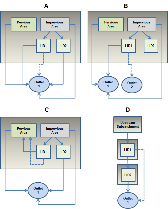
Figure 6‑6 Different options for placing LID controls
LID computations are a sub-procedure of SWMM's runoff calculations. They are made at each runoff time step, for each subcatchment that contains LID controls, immediately after the runoff from the non-LID portions (both pervious and impervious) of the subcatchment have been found and before any groundwater calculations are made (see Section 3.4 of Volume I). The computations for an individual LID unit include the following four steps:
The process of determining the inflow to the LID unit in step 1 depends on whether the unit comprises only a portion of its subcatchment's area or if it occupies the entire subcatchment. In the former case the runoff rate *q0* treated by the unit can be computed as:
\[q_{0} = q_{imp}F_{out}R_{LID}\]
(6-61)
where
*qimp* = total impervious area runoff rate (ft/sec),
*Fout* = fraction of impervious area runoff routed to the subcatchment's outlet,
*RLID* = capture ratio of the LID unit.
Note that *Fout* accounts for the possibility that the user has assigned some portion of the subcatchment's impervious area runoff to be re-routed onto its pervious area using SWMM's overland flow re-routing option (explained in Section 3.6 of Volume I). When there is no internal re-routing (or disconnecting) of impervious area *Fout* is equal to 1.0. Also introduced is a new parameter, the LID unit's capture ratio *RLID*. It is defined as the amount of the subcatchment's impervious area that is directly connected to the LID unit divided by the area of the LID unit itself.
When a single LID unit occupies the entire subcatchment *q0* is comprised of any external overland flow routed onto the subcatchment. Such flow can consist of runoff originating from other upstream subcatchments as well as any underdrain flow from other LID units routed onto the subcatchment.
Step 2 of the computational procedure evaluates the flux terms on the right hand side of the governing continuity equation for each layer of the LID unit being analyzed. These terms depend on the current moisture level stored in each layer. Section 6.2 has discussed in detail how each flux term is computed. Recall that evapotranspiration is evaluated first, moving from the top to the bottom of the LID unit. The remaining flux terms are then evaluated in the opposite direction, moving from the bottom to the topmost layer of the unit.
Step 3 integrates the governing continuity equations over a single time step to find new values for the moisture content in each of the LID unit's layers. Let x be the vector of the layer moisture contents, where x = [*φ1d1, D2θ2, φ3d3, D4(1-F4)θ4*], and let Γ = [*Γ1, Γ2, Γ3, Γ4*] be the vector of the net flux (inflow minus outflow) of water through each layer (i.e., the right hand side value of each layer's continuity equation). If a particular layer i does not apply to a given LID unit, such as the soil layer for a rain barrel, then both *xi* and *Γi*would be zero. Now the flow continuity equations can be written more compactly as:
\[\frac{\partial\mathbf{x}}{\partial t} = \mathbf{\Gamma}(\mathbf{x(}t\mathbf{)})\]
(6-62)
where in general Γ is a nonlinear function of x.
This system of equations can be solved numerically by using the trapezoidal method (Ascher and Petzold, 1998) to discretize them in time as follows:
\[\mathbf{x}(t + \mathrm{\Delta}t) = \mathbf{x}(t)\mathbf{+}\left\lbrack \Omega\mathbf{\Gamma}(\mathbf{x}(t + \mathrm{\Delta}t)\mathbf{+ (}1 - \Omega\mathbf{)\Gamma}(\mathbf{x}(t)\mathbf{)} \right\rbrack\mathbf{\mathrm{\Delta}}t\]
(6-63)
where Ω = 0.5 and ∆t is the wet hydrologic time step used for computing runoff. (See Section 3.5 of Volume I for a discussion of SWMM's runoff time steps.) This equation makes the new moisture content in the LID unit equal to the previous moisture content plus the average net flow volume occurring over the time step. At time 0 the moisture content in the LID unit's soil and storage layers is set to a user-supplied percent of saturation while the other layer moisture levels 00start at 0.
Because ***Γ**(x(t+∆t))* appearing on the right hand side of Equation 6-55 depends on the unknown new moisture content, an iterative method must be used to solve the equation. Let ***x**(t+∆t)ν* be the estimate of ***x**(t+∆t)* at iteration ν, where initially ***x**(t+∆t)0 = x(t)*. (Note that ν is an iteration counter, not a power.) Then for iteration ν+1 the new estimate of ***x**(t+∆t)* is:
\[\mathbf{x}{(t + \mathrm{\Delta}t)}^{\nu + 1}\mathbf{= x}(t)\mathbf{+}\left\lbrack \Omega\mathbf{\Gamma}(\mathbf{x}(t + \mathrm{\Delta}t)^{\nu}\mathbf{+ (}1 - \Omega\mathbf{)\Gamma}(\mathbf{x}(t)\mathbf{)} \right\rbrack\mathbf{\mathrm{\Delta}}t\]
(6-64)
with the iterations stopping when the change in ***x**(t+∆t)* is sufficiently small. SWMM uses a tolerance of 0.00328 feet (or 1.0 millimeter) as a stopping tolerance.
If Ω is chosen as 0, then Equation 6-64 becomes equivalent to the Euler method and thus:
\[\mathbf{x}(t + \mathrm{\Delta}t) = \mathbf{x}(t)\mathbf{+ \Gamma}(\mathbf{x}(t))\mathbf{\mathrm{\Delta}}t\]
(6-65)
which can be solved directly without resorting to any iterative scheme. Numerical testing has shown that the simpler Euler method works well with all types of controls except for vegetative swales. The latter requires the iterative trapezoidal method with a Ω of 0.5 to produce results with acceptable continuity errors.
When using either Equation 6-64 or 6-65 to update the LID unit's moisture state at each time step, the following lower and upper physical limits on moisture levels must be enforced:
\[0 \leq d_{1} \leq D_{1}\]
\[\theta_{WP} \leq \theta_{2} \leq \phi_{2}\]
\[0 \leq d_{3} \leq D_{3}\]
\[0 \leq \theta_{4} \leq \phi_{4}\]
Finally, Step 4 merges the outflows from the LID unit with those of the subcatchment as a whole. Any infiltration into the native soil produced by the LID unit is added onto the total infiltration for the subcatchment, which is eventually passed onto SWMM's groundwater module. Any underdrain flow from the LID unit is kept track of separately, so that it can be routed to its designated destination (either another subcatchment or some location in the conveyance system). It is not included as part of the subcatchment's reported surface runoff. Any surface runoff or overflow from the unit \(\left( q_{1}A \right)\) is added to the subcatchment's total runoff flow rate, except if the unit's outflow has been designated for return to the subcatchment's pervious area. In the latter case a separate account is kept of the total return flow and the LID surface flow is added to it.
As regards to water quality, no explicit changes in constituent concentrations are computed as runoff passes through or over an LID control. A subcatchment's pollutant washoff concentration is computed as described in Section 4.3, as if no LID controls existed. Any surface outflow or underdrain flow from each of the subcatchment's LID controls is assigned this concentration.
There are two exceptions to this convention. One applies when the LID units take up less than the full area of the subcatchment and a pollutant has a non-zero rainfall concentration. In that case the washoff load from the non-LID portion of the subcatchment (which already accounts for any wet deposition) is combined with the direct rainfall load from the LID areas to arrive at a modified outflow concentration:
\[C_{out} = \frac{\left\lbrack \left( C_{out}Q_{out} \right)_{non - LID} + C_{ppt}iA_{LID} \right\rbrack}{Q_{out,non - LID} + iA_{LID}}\]
(6-66)
where
*Cout* = concentration of a pollutant in the subcatchment's outflow streams after LID treatment (mass/L),
*Cout,non-LID* = concentration of a pollutant in the subcatchment's outflow streams prior to LID treatment (mass/L),
*Qout,non-LID* = surface runoff flow rate leaving the subcatchment prior to any LID treatment (cfs),
*Cppt* = concentration of the pollutant in rainfall (mass/L),
i = rainfall rate (ft/sec),
*ALID* = total surface area of all LID units in the subcatchment (ft2).
The second exception is when a single LID unit occupies its entire subcatchment. In that case there would be no washoff load generated by any non-LID surfaces and the pollutant concentration in the unit's outflow streams would equal that of its inflow stream. Thus for any particular pollutant,
\[C_{out} = \frac{\left( \left( \frac{W_{runon}}{28.3} \right) + C_{ppt}iA_{LID} \right)}{Q_{runon} + iA_{LID}}\]
(6-67)
where *Qrunon* is the combined runoff flow rate (cfs) of all upstream subcatchments routed onto the LID subcatchment, W~runon~ is the total pollutant load (mass/sec) contained in this runoff inflow, and the factor 28.3 converts from cubic feet to liters.
Thus although an LID control does not modify the concentration of a water quality constituent it sees in its inflow stream, it does reduce the total pollutant load passed on to downstream locations in direct proportion to the reduction in runoff it produces. When a storm is completely captured by an LID unit its effective pollutant removal efficiency is 100 percent.
The variety of LID controls modeled by SWMM introduces a significant number of design variables and parameters that must be assigned values by the user. These include sizing parameters (surface area, layer depths, and capture ratio), surface parameters (freeboard depth, outflow face width, slope, and roughness), soil parameters (moisture limits and hydraulic conductivity), pavement parameters (void ratio and permeability), storage parameters (void ratio and native soil conductivity), drain parameters (discharge coefficient and exponent, roof drain capacity, and drain mat roughness), and clogging parameter. Because of the high interest and acceptance of LID, many local and state agencies have prepared design manuals that recommend ranges for many key parameters. Table 6-1 lists a selection of these manuals, all available online. Unless otherwise noted, these manuals served as the source of the LID parameter values described in the sub-sections that follow.
Table 6-2 lists ranges of parameter values for bio-retention cells and rain gardens, expressed in their typical US units of inches and hours. They are internally converted to feet and seconds for use in the governing conservation equations.
The soil moisture limits in the table are based on ranges computed for sand, loamy sand, and sandy loam textures using the SPAW model (Saxton and Rawls, 2006) with organic contents ranging between 2.5 and 8%. The model can be used to estimate specific limits from knowledge of a soil's sand, clay and organic content. For example, a typical engineered soil might consist of 85% sand, 5% clay and 5% organic matter by weight. Using the SPAW calculator for this soil produces the characteristics listed in Table 6-3. The percolation decay constant HCO was estimated by using the calculator to compute hydraulic conductivity *K2* for a range of moisture contents θ and then regressing \(- ln\left( \frac{K_{2}}{K_{2S}} \right)\) against \(\phi_{2} - \theta\) to find a best-fit value for HCO. The equation used to estimate suction head was introduced in Section 4.4 of Volume I.
Table 6-1 Design manuals used as sources for LID parameter values
| Organization | Manual Title | Year | URL |
|---|---|---|---|
| Prince Georges County Maryland | Low-Impact Development Design: An Integrated Design Approach | 1999 | http://water.epa.gov/polwaste/green/upload/lidnatl.pdf |
| Denver Urban Drainage and Flood Control District | Urban Storm Drainage Criteria Manual, Volume 3 Best Management Practices | 2010 | http://udfcd.org/wp-content/uploads/uploads/vol3%20criteria%20manual/USDCM%20Volume%203.pdf |
| Toronto and Region Conservation Authority | Low Impact Development Stormwater Management Planning and Design Guide | 2010 | http://www.creditvalleyca.ca/wp-content/uploads/2014/04/LID-SWM-Guide-v1.0_2010_1_no-appendices.pdf |
| Washington State University Extension | Low Impact Development Technical Guidance Manual for Puget Sound | 2012 | http://www.psp.wa.gov/downloads/LID/20121221_LIDmanual_FINAL_secure.pdf |
| District of Columbia | Stormwater Management Guidebook | 2013 | http://doee.dc.gov/swguidebook |
| Philadelphia Water Department | Stormwater Management Guidance Manual, Version 2.1 | 2014 | http://www.pwdplanreview.org/upload/pdf/Full%20Manual%20%28Manual%20Version%202.1%29.pdf |
| University of New Hampshire Stormwater Center | UNHSC Design Specifications for Porous Asphalt Pavement and Infiltration Beds | 2014 | http://www.unh.edu/unhsc/sites/unh.edu.unhsc/files/pubs_specs_info/unhsc_pa_spec_10_09.pdf |
| NY State Department of Environmental Conservation | Stormwater Management Design Manual | 2015 | http://www.dec.ny.gov/docs/water_pdf/swdm2015entire.pdf |
Table 6-2 Typical ranges for bio-retention cell parameters
| Parameter | Range |
|---|---|
| Maximum Freeboard, inches (*D1*) | 6 – 12 |
| Surface Void Fraction (*φ1*) | 0.8 – 1.0 |
| Soil Layer Thickness, inches (*D2*) | 24 – 48 |
| Soil Properties: | |
| > Porosity (*φ2*) | 0.45 – 0.6 |
| > Field Capacity (*θFC*) | 0.15 – 0.25 |
| > Wilting Point *(θWP*) | 0.05 – 0.15 |
| > Saturated Hydraulic Conductivity, in/hr (*K2S*) | 2.0 – 5.5 |
| > Wetting Front Suction Head, inches (*ψ2*) | 2 – 4 |
| > Percolation Decay Constant (HCO) | 30 – 55 |
| Storage Layer Thickness, inches (*D3*) | 6 – 36 |
| Storage Void Fraction (*φ3*) | 0.2 – 0.4 |
| Capture Ratio (*RLID*) | 5 – 15 |
Table 6-3 Soil characteristics for a typical bio-retention cell soil
| Soil Property | Value |
|---|---|
| Porosity (*φ2*) | 0.52 |
| Field Capacity (*θFC*) | 0.15 |
| Wilting Point *(θWP*) | 0.08 |
| Saturated Hydraulic Conductivity, in/hr (*K2S*) | 4.7 |
| Percolation Decay Constant (HCO) | 39.3 |
| Wetting Front Suction Head, inches (*ψ2 = 3.23(K2S*)-0.328) | 1.9 |
Typical ranges of parameter values for Green Roofs are listed in Table 6-4. These are for extensive green roofs of relatively shallow thickness.
Table 6-4 Typical ranges for green roof parameters
| Parameter | Range |
|---|---|
| Maximum Freeboard, inches (*D1*) | 0 – 3 |
| Surface Void Fraction (*φ1*) | 0.8 – 1.0 |
| Soil Layer Thickness, inches (*D2*) | 2 – 6 |
| Soil Parameters: | |
| > Porosity (*φ2*) | 0.45 – 0.6 |
| > Field Capacity (*θFC*) | 0.3 – 0.5 |
| > Wilting Point (*θWP*) | 0.05 – 0.2 |
| > Plant Available Water (*θFC* - *θWP*) | 0.25 – 0.3 |
| > Saturated Hydraulic Conductivity, in/hr (*K2S*) | 40 – 140 |
| > Wetting Front Suction Head, inches (*ψ2*) | 2 – 4 |
| > Percolation Parameter (HCO) | 30 – 55 |
| Drainage Layer Thickness, inches (*D3*) | 0.5 – 2 |
| Drainage Layer Void Fraction (*φ3*) | 0.2 – 0.4 |
| Drainage Layer Roughness (*n3*) | 0.01 – 0.03 |
| Capture Ratio (*RLID*) | 0 |
The "soil" used as a growth media for green roofs is very different from naturally occurring soils. It is an engineered mixture of aggregate (such as expanded slate or shale, pumice, or zeolite), sand, and organic matter producing a light weight product with high porosity and water holding capacity. There is a limited amount of information on the standard agronomic properties of such mixtures. The moisture limits and conductivity values listed in Table 6-4 are based on a literature review provided by Perelli (2014). When compared to the properties for bio-retention cell media, the green roof media's hydraulic conductivity is much higher. The ranges for suction head and the percolation parameter were defaulted to those typical of loam and sandy loam soils. The capture ratio for a green roof should be 0 since its only inflow is direct rainfall.
Suggested ranges for the parameters associated with infiltration trenches are listed in Table 6-5. Because there is no soil layer to slow down and retain water in excess of gravity drainage, the trench acts as a simple "storage pit" whose change in stored volume over a given time step is simply the difference between the captured runoff/rainfall rate entering through its surface and the rate of exfiltration leaving through its bottom (assuming no underdrain).
Table 6-5 Typical ranges for infiltration trench parameters
| Parameter | Range |
|---|---|
| Maximum Freeboard, inches (*D1*) | 0 – 12 |
| Surface Void Fraction (*φ1*) | 1.0 |
| Storage Layer Thickness, inches (*D3*) | 36 – 144 |
| Storage Void Fraction (*φ3*) | 0.2 – 0.4 |
| Contributing Area, acres | 1 – 5 |
| Capture Ratio (*RLID*) | 5 – 20 |
Table 6-6 lists typical parameter ranges for permeable pavement installations. The maximum storage height on the surface layer, *D1*, now represents the depth of depression storage on the pavement surface. Its suggested range is characteristic of impervious surfaces in general (ASCE, 1992). The pavement layer properties in the table distinguish between continuous concrete or asphalt pavement systems and block paver systems.
UNHSC (2009) recommends that the optional sand filter layer be composed of coarse sand/fine gravel (bank run gravel). It aids in pollutant removal and in slowing down the movement of water through the unit. Because of the very high conductivity of permeable pavement, with no sand layer present the unit acts in the same manner as an infiltration trench whose change in water level over each time step is simply the difference between the applied surface inflow rate and the exfiltration rate out of the bottom (assuming no underdrain).
Table 6-6 Typical ranges for permeable pavement parameters
| Parameter | Range |
|---|---|
| Surface Depression Storage, inches (*D1*) | 0 – 0.1 |
| Surface Void Fraction (*φ1*) | 1.0 |
| Pavement Thickness, inches (*D4*) | 3 – 8 |
| Continuous Pavement: | |
| > Porosity (*φ4*) | 0.15 – 0.25 |
| > Permeability, in/hr (*K4*) | 28 – 1750 |
| > Surface Opening Fraction (*1 – F4*) | 0 |
| Block Pavers: | |
| > Porosity (*φ4*) | 0.1 – 0.4 |
| > Permeability, in/hr (*K4*) | 5 – 150 |
| > Surface Opening Fraction (*1 – F4*) | 0.08 – 0.10 |
| Sand Filter Layer: | |
| > Thickness, inches (*D2*) | 8 – 12 |
| > Porosity (*φ2*) | 0.25 – 0.35 |
| > Field Capacity (*θFC*) | 0.15 – 0.25 |
| > Wilting Point *(θWP*) | 0.05 – 0.10 |
| > Saturated Hydraulic Conductivity, in/hr (*K2S*) | 5 – 30 |
| > Wetting Front Suction Head, inches (*ψ2*) | 2 – 4 |
| > Percolation Parameter (HCO) | 30 – 55 |
| Storage Layer Thickness, inches (*D3*) | 6 – 36 |
| Storage Void Fraction (*φ3*) | 0.2 – 0.4 |
| Capture Ratio (*RLID*) | 0 – 5 |
The Rain Barrel LID control can be used to model both rain barrels and cisterns. Rain barrels are typically 50 to 100 gallons in capacity and are used at individual home lots to collect roof runoff for possible landscape irrigation. Cisterns have much larger capacity, typically from 250 to 30,000 gallons, used to harvest rainwater from both homes and commercial facilities for non-potable indoor use. The parameters required for Rain Barrels/Cisterns are the height of the storage vessel (*D3*), its volume (from which its surface area A~LID~ can be derived), its drain parameters, and possibly its drain delay time.
The height and volume of the rain barrel/cistern would be determined by commercially available sizes. The drain offset is typically 6 inches from the bottom (to trap sediment). Alternatively, one could use an offset of 0 and reduce the vessel height accordingly.
The drain flow parameters can be established from the orifice equation (Equation 6-38). The flow exponent would be 0.5 and the flow coefficient would be 4.8 times the ratio of the drain diameter to the barrel diameter squared. The latter quantity has units of ft0.5/sec. To convert to the in0.5/hr (or mm0.5/hr) used in SWMM's input data set multiply by 12,471 (or 62,768).
As an example, a 2-foot diameter rain barrel with a 3/4 inch spigot would have a drain flow coefficient of 4.8 × (0.75 / (2×12))2 × 12,471 = 58.5 in0.5/hr. This is high enough to drain 4 feet of captured water (94 gallons) in less than 15 minutes. A slower release rate for landscape irrigation can be achieved by leaving the spigot valve only partially open or by using a soaker hose. This action can be simulated by using a reduced drain diameter when computing a drain flow coefficient.
The drain delay time is the period of time after rainfall ceases until the rain barrel is allowed to drain. If the delay time is set to 0 then the drain line is considered to be always open. This option might be appropriate for modeling rainwater harvesting with larger cisterns. Otherwise a choice of delay time will depend on what assumptions one makes about homeowner behavior.
The parameters required for rooftop disconnection are the length of the flow path for roof runoff (the inverse of the W1/A1 term in Equation 6-21), the roof slope, the roughness coefficient for the roof surface, the depression storage depth of the roof's surface, and the flow capacity of the roof drain system (*q3max*).
The flow path length and its slope are obtained directly from the roof's dimensions. Roughness coefficients for roofing material would be similar to those for asphalt and clay tile, 0.013 to 0.016. Depression storage would range from 0.05 to 0.1 inches with sloped roofs at the low end of this range and flat roofs having possibly higher values. The flow capacity of the roof's gutters in ft/sec can be estimated from the following equations (Beij, 1934):
for semicircular gutters
\[q_{3max} = 0.52\frac{w_{g}^{2.5}}{A_{r}}\]
(6-68)
for rectangular gutters
\[q_{3max} = 7.75\left( \frac{d_{g}}{w_{g}} \right)^{1.6}\left( \frac{w_{g}}{L_{g}} \right)^{0.3}w_{g}^{2.5}/A_{r}\]
(6-69)
where *wg* is the gutter width in feet, d~g~ is the gutter depth in feet, *Ar* is the area of the roof serviced by the gutter in square feet, and *Lg* is the length of the gutter in feet. To convert *q3max* to the in/hr or mm/hr required by the SWMM 5 input format, multiply by 43,200 or 1,097,280, respectively.
Typical values for the parameters associated with vegetative swales are listed in table 6-7. The top width of the swale at full depth (*W1*) equals \(W_{X} + 2D_{1}S_{X}\). The maximum surface area covered by the swale (A~LID~) can be found by multiplying *W1* by the length of the swale.
Table 6-7 Typical ranges for vegetative swale parameters
| Parameter | Range |
|---|---|
| Maximum Depth, feet (*D1*) | 0.5 – 2.0 |
| Surface Void Fraction (*φ1*) | 0.8 - 1.0 |
| Bottom Width, feet (*WX*) | 2.0 – 8.0 |
| Surface Slope, percent (*S1*) | 0.5 – 3.0 |
| Side Slope, horizontal : vertical (*SX*) | 2.5 : 1 – 4 : 1 |
| Surface Roughness (*n1*) | 0.03 – 0.2 |
| Capture Ratio (*RLID*) | 5 – 10 |
Underdrains are either recommended or required when the natural soil infiltration rate is insufficient to prevent the LID unit from flooding. There are three user-supplied parameters that describe underdrain flow: a discharge coefficient (*C3D*), a discharge exponent (*η3D*), and a drain offset height (*DD3*). While the drain offset is part of the cell's physical design, the discharge coefficient and exponent must be inferred from the hydraulics of underdrain flow. There are several approaches that can be used for this:
To use option 1, the full flow capacity of the drain pipe can be computed from the Manning equation as follows:
\[Q_{full} = \left( \frac{0.464}{n_{pipe}} \right)S_{pipe}^{0.5}D_{pipe}^{2.67}\]
(6-70)
where *Qfull* is the flow rate (cfs), *npipe* is the roughness coefficient for the pipe's material, *Spipe* is the slope at which the pipe is laid (ft/ft), and *Dpipe* is the pipe's diameter (ft). To convert this value into a set of underdrain discharge parameters, set the drain exponent *η3D* to zero and the drain coefficient *C3D* to
\[C_{3D} = \frac{N_{pipe}Q_{full}}{A_{LID}}\]
(6-71)
where *Npipe* is the number of drain pipes in the unit and *ALID* is the area (ft2) of the unit. Because *η3D* is zero, the units of *C3D* are ft/sec. To convert these to the in/hr or mm/hr required by the SWMM 5 input format, multiply by 43,200 or 1,097,280, respectively.
As an example, using this method to specify the underdrain parameters for two 4-inch diameter plastic drain lines with roughness of 0.01 placed at a 0.5% slope in a 1,000 sq. ft. bio-retention cell would produce a drain coefficient equal to
\[C_{3D} = \frac{2\left( \frac{0.464}{0.01} \right){(0.005)}^{0.5}{(\frac{4}{12)}}^{2.67}}{1000} = 0.00035\ \frac{ft}{\sec} = 15\ \frac{in}{hr}\]
Once the water height in the storage layer reaches the drain's offset height, any inflow from percolation out of the soil layer will immediately flow out of the underdrain as long as its flow rate is below 15 in/hr (as per Equation 6-8) and the storage volume above the offset height will never be used.
For option 2, one can assume that the standard orifice equation can replace the underdrain flow expression Equation 6-7 so that:
\[q_{3} = C_{3D}\left( h_{3} \right)^{0.5}\]
(6-72)
where the discharge exponent *η3D* has been set to 0.5 and the discharge coefficient now becomes:
\[C_{3D} = 0.6\sqrt{2g}\left( \frac{A_{slot}}{A_{LID}} \right)\]
(6-73)
with *Aslot* being the total area (ft2) of the slots in the drain pipe and g the acceleration of gravity (32.2 ft/sec2). Note that the units of *C3D* are ft0.5/sec so when used in Equation 6-63 the resulting underdrain flux has units of ft/sec (or cfs/ft2). To convert *C3D* to in0.5/hr, which are the US units used in the program's input, one would multiply by 12,471. To convert to mm0.5/hr for SI units, multiply by 62,852.
The ratio of the total slot area to LID area can be determined from the dimensions of a slot, the spacing between slots along the drain pipe, and the spacing between individual drain pipes:
\[\frac{A_{slot}}{A_{LID} =}\frac{N_{pipe}{N_{slot}A}_{slot}}{\left( N_{pipe} + 1 \right)\Delta_{pipe}}\]
(6-74)
where
*Npipe* = number of underdrain pipes
*Nslot* = number of slots per length of pipe (ft-1)
*Aslot* = area of a single slot (ft2)
*∆pipe* = spacing between pipes (ft)
As an example, consider an underdrain system consisting of two slotted pipes with inlet area of 1 in2 per foot of pipe spaced 50 ft apart. The area ratio used to compute *C3D* would be:
\[\frac{A_{slot}}{A_{LID} = \frac{2 \times \left( \frac{1}{144} \right)}{(3 \times 50) = 0.0000926}}\]
Using this value in Equation 6-64 to compute *C3D* produces:
\[C_{3D} = 0.6 \times \sqrt{64.4} \times 0.0000926 = 0.00045\ \frac{{ft}^{0.5}}{\sec} = 5.5\ \frac{{in}^{0.5}}{hr}\]
Regarding the third option for underdrain parameters, the underdrain flow expression can again be replaced by the standard orifice equation, this time applied to the discharge point of the underdrain system (such as the outlet of a pipe manifold fitted with a cap orifice):
\[C_{3D} = 0.6\sqrt{2g}\left( \frac{A_{out}}{A_{LID}} \right)\]
(6-75)
where Aout is the cross-sectional area (ft2) of the outlet fitting. The same conversion factors described previously would be used to convert *C3D*from ft0.5/sec to either in0.5/hr or mm0.5/hr.
Applying this approach to the previously mentioned pair of 4-inch diameter drain pipes servicing a 1,000 ft2 cell without any flow restriction would result in a *C3D* value of 10.5 in0.5/hr. This is much higher than the 5.5 in0.5/hr based on inlet control. Hence the latter number would be used for *C3D* under these particular circumstances. If the two underdrain pipes were connected by a tee fitting to a single 4-inch diameter outflow then the discharge coefficient would be 5.25 in0.5/hr and the drain would operate under outlet control.
Because clogging is a long-term process, it would only apply to simulations of several months or more duration. SWMM assumes that clogging (i.e., reduction of infiltration rates for permeable pavement systems and infiltration trenches) proceeds at a constant rate proportional to the number of void volumes that the LID unit treats over time. The clogging rate constant (or clogging factor CF) can be computed from the number of years *Tclog* it takes to fractionally reduce an infiltration rate to a degree *Fclog*. For example, a CF for permeable pavement can be estimated from:
\[{CF}_{4} = \frac{I_{a}\left( 1 + R_{LID} \right)T_{clog}}{\phi_{4}D_{4}\left( 1 - F_{4} \right)F_{clog}}\]
(6-76)
where *Ia* is the annual volume of rainfall in inches, *RLID* is the unit's capture ratio, *φ4* is the porosity of the pavement layer, *D4* is the thickness of the pavement layer, and *F4* is the fraction of the surface area covered by impermeable pavers. A similar expression would apply to the CF of an infiltration trench's storage layer using the layer's porosity and thickness in the expression with *F4* set to 0.
For permeable pavement, the rate at which clogging proceeds depends on many factors, such as the type of permeable pavement system employed, the pore sizes in the pavement or in the fill material between paver blocks, the amount and size of the particulate matter in the runoff it treats, and the amount of vehicular traffic passing over it. Perhaps the most important factor for both permeable pavement and infiltration trenches is the capture ratio since that will affect how much solids loading the unit receives over a given span of years. That is, with all other factors being equal, an LID unit with a higher capture ratio will clog in less time than one with a lower capture ratio.
Kumar et al. (2016) measured reductions in infiltration rates of 71 to 85 % after 3 years for a permeable pavement parking lot. Pitt and Voorhees (2000) quote a possible 50 % drop in permeable pavement permeability in 3 years. In simulated loading conditions, Yong et al. (2013) found that permeable asphalt pavement became completely clogged in 8 to 12 years. Bergman et al. (2011) found a 74 % drop in infiltration rate over 15 years for a pair of infiltration trenches in Copenhagen.
A numerical example will help demonstrate how SWMM is able to model the dynamic behavior that LID controls exhibit during a rainfall event. Consider a bio-retention cell that captures all of the runoff from a parking lot. It consists of a 24 inch soil layer above a 12 inch gravel reservoir and has a 6-inch high berm surrounding it. The growth medium in the soil layer is the same 85% sand, 5% clay and 5% organic matter blend whose properties were listed previously in Table 6-3 (porosity of 0.52, field capacity of 0.15, wilting point of 0.08, saturated hydraulic conductivity of 4.7 in/hr, suction head of 1.9 inches, and percolation decay constant of 39.3). The void fraction of the gravel storage layer is 0.4 and the exfiltration rate out of this layer into the native soil is 0.4 in/hr. Initially it is assumed that the bio-retention cell is not equipped with an underdrain.
The parking lot is completely impervious and is modeled so that all rainfall becomes immediate runoff. The bio-retention cell takes up 5 % of the total catchment area. Thus its Capture Ratio is (1 – 0.05) / 0.05 = 19. The total storage volume contained in the bio-retention cell is 6 inches of above ground surface storage plus 24 × (0.52 – 0.08) inches of soil pore volume plus 12 × 0.4 inches of gravel volume for a total of 21.36 inches. Considering the unit's capture ratio of 19 plus the area of the unit itself translates into a capacity of 21.36 / (19 + 1) = 1.07 inches for the entire catchment area. Thus it should be capable of completely capturing and infiltrating all storms at or below this depth. This is just an estimate since it ignores the effect that the 0.4 in/hr exfiltration rate out of the bottom of the unit has in making more storage available as an event unfolds.
The parking lot and bio-retention cell were subjected to the 1 inch storm event depicted in Figure 6-7. This is an actual event recorded at a rain gage in Philadelphia, PA during the month of May. The potential evaporation rate for that time of year was 0.18 in/day. SWMM 5 was used to compute the hydrologic response of the parking lot and its LID control to this storm event over a 48-hour period starting with completely dry conditions. Results for the bio-retention cell are shown in Figures 6-8 and 6-9. Figure 6-8 shows the variation over time of the surface inflow, soil layer percolation, and storage layer exfiltration. Figure 6-9 shows how the moisture level within each layer, as a percentage of its full storage capacity, varies with time.
Figure 6‑7 Storm event used for the LID example
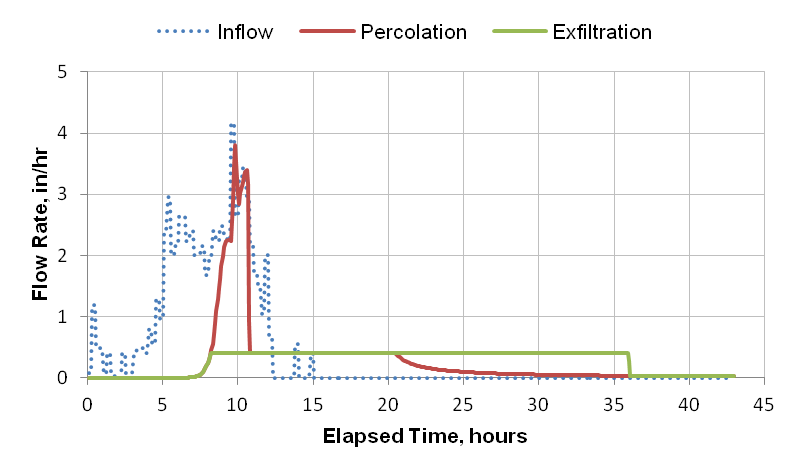
Figure 6‑8 Flux rates through the bio-retention cell with no underdrain
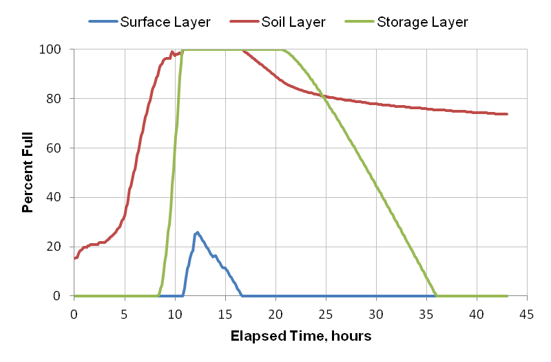
Figure 6‑9 Moisture levels in the bio-retention cell with no underdrain
The bio-retention cell is able to completely capture this 1-inch storm. Although both the storage and soil zones become saturated and some surface ponding occurs (up to a maximum 0.25 × 6 = 1.5 inches), no runoff is produced. The dynamics of flow through the unit can be broken up into five distinct phases:
For the first 5 hours of the storm event the soil fills with water up to its field capacity of 0.15 (29% of saturation). During this time the soil layer accepts all inflow to the unit without sending any outflow to the storage layer.
During the next 6 hours as the unit continues to receive inflow, water begins to percolate out of the soil layer and into the storage layer at an increasing rate. For the first 3 hours of this period, while the percolation rate is below the bottom exfiltration rate, all of this water leaves the unit and keeps the storage layer dry. Eventually the soil moisture content becomes high enough so that the percolation rate exceeds the exfiltration rate and the storage layer fills in a matter of 3 hours. During this entire phase the unit is still able to accept all of the inflow as shown by the absence of any ponded surface water.
After approximately 11 hours both the soil and storage layers have become full. At this point even though the soil conductivity has risen above 4 in/hr, it cannot transmit water any faster than the full storage layer can exfiltrate it at only 0.4 in/hr. During the next 4 hours as the unit continues to receive inflow while full, the excess ponds atop the surface.
Once inflow to the unit ceases at about 15 hours it begins to drain and water levels recede from the top on down. Surface ponding is gone by 16.5 hours. Then the soil begins to drain down at a rate still limited by the slower bottom exfiltration rate since the storage layer remains full. At about hour 21 the soil percolation rate becomes less than the exfiltration rate and the storage layer begins to empty. It then takes another 15 hours for the storage layer to drain down completely.
After the storage layer has completely drained, water continues to drain out of the soil layer at a rate lower than the bottom exfiltration rate, so all of it infiltrates into the native soil. This continues until the soil's field capacity moisture is reached. After that, the soil will continue to dry by evapotranspiration until its wilting point is reached.
Now consider what happens when an underdrain is added to the bio-retention cell. The drain is placed at the top of the storage layer so that the layer's full storage capacity can be utilized. It is assumed to be over-designed so its discharge coefficient is assigned a very large value. The resulting time history of moisture content throughout the cell with the underdrain is shown in Figure 6-10. The drain has prevented any inflow from ponding on top of the unit. As shown in Figure 6-11, the drain carries flow only during the period of time that the storage layer is full. Because it is oversized, it can accept the full amount of water remaining from soil percolation after the bottom exfiltration is accounted for. Compare this with the case of no drain in Figure 6-8, where the soil percolation rate is limited by the exfiltration rate during the time that the storage layer is full.
The total volume of flow carried away by the underdrain is about 14 % of the total storm volume. If this flow is sent to a storm sewer which is typically the case, then the bio-retention cell can no longer be said to have fully captured and eliminated runoff from this 1-inch storm.
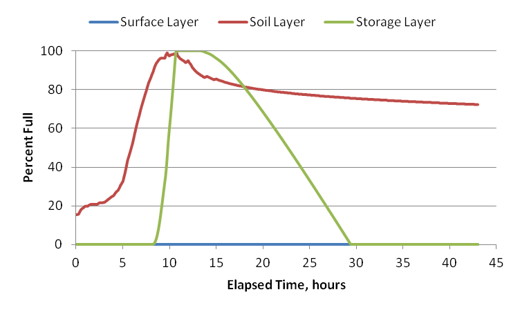
Figure 6‑10 Moisture levels in the bio-retention cell with underdrain
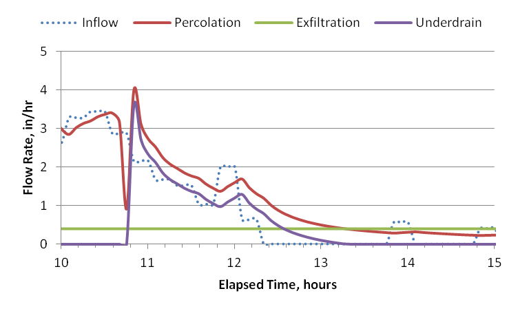
Figure 6‑11 Flux rates through the bio-retention cell with underdrain
 1.13.2