 |
OpenSWMM Engine
6.0.0-alpha.4
Data-oriented, plugin-extensible SWMM Engine (6.0.0-alpha.4)
|
|
OpenSWMM Engine
6.0.0-alpha.4
Data-oriented, plugin-extensible SWMM Engine (6.0.0-alpha.4)
|
Water quality constituents in surface runoff and from other external sources will typically be transported through a conveyance system until they are discharged into a receiving water body, a treatment facility, or some other type of destination (such as back to the land surface for irrigation purposes). Figure 5-1 shows how SWMM represents this conveyance system as a network of Nodes and Links. Nodes are points that represent simple junctions, flow dividers, storage units, or outfalls. Links connect nodes to one another with conduits (pipes and channels), pumps, or flow regulators (orifices, weirs, or outlets). Inflows to nodes can come from surface runoff, groundwater interflow, RDII (rainfall dependent inflow/infiltration), sanitary dry weather flow, or from user-defined time series. Pollutants can be removed by natural decay processes as they flow through conduits and storage nodes, and they can also be reduced by treatment processes applied at both non-storage nodes (e.g., high-rate solids separators) and storage nodes (e.g., physical sedimentation). This chapter describes how SWMM computes pollutant concentrations within all conduits and nodes of the conveyance network at each computational time step after its hydraulic state has been determined. The latter consists of the flow rate and volume of water in each link and the volume of water within each storage node. The methods used to obtain this hydraulic solution are described in Volume II of this manual.
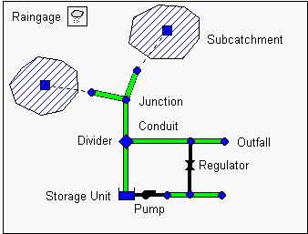
Figure 5‑1 Representation of the conveyance network in SWMM
The one-dimensional transport of dissolved constituents along the length of a conduit (a pipe or natural channel) is described by the following conservation of mass equation (Martin and McCutcheon, 1999):
\[\frac{\partial c}{\partial t} = - \frac{\partial(uc)}{\partial x} + \frac{\partial}{\partial x}\left( D\frac{\partial c}{dx} \right) + r(c)\]
(5-1)
where c = constituent concentration (ML-3), u = longitudinal velocity (LT-1), D = longitudinal dispersion coefficient (L2/T), r(c) = reaction rate term (ML-3T-1)), x = longitudinal distance (L), and t = time (T). Note that c is a continuous function of both distance x and time t. In general, c can be a vector of constituents in which case a separate Equation 5-1 would apply for each constituent and the reaction rate r could be a function of more than one constituent. The first term on the right hand side of Equation 5-1 represents advective transport where the constituent mass within a parcel of water moves along the conduit at the same velocity as the bulk fluid. The second term represents longitudinal dispersion where, due to velocity and concentration gradients, some portion of the mass inside a parcel mixes with the contents of parcels on either side of it. The final term represents any reactions that modify the concentration within a parcel regardless of any fluid motion.
A set of boundary and initial conditions is needed to solve Equation 5-1. In a conveyance network of the type modeled by SWMM the boundary conditions would be the concentrations at the nodes at either end of a conduit. For a simple junction node that has no storage volume associated with it the instantaneous concentration is simply the instantaneous flow weighted average concentration of all inflows that the junction receives:
\[c_{Nj} = \frac{\sum_{i \rightarrow j}^{}{c_{L2i}q_{2i} + W_{j}}}{\sum_{i \rightarrow j}^{}q_{2i} + Q_{j}}\]
(5-2)
where *cNj* is the concentration at node j, *cL2i* is the concentration at the end of link i that connects to node j, *q2i* is the flow rate at the end of link i, *Wj* is the mass flow rate of any direct external source of constituent to node j, *Qj* is the flow rate of the external source, and the summations are over all links that have flow directed into node j. For a storage node where it is assumed that the contents of the stored volume are completely mixed, the uniform concentration within the node is governed by the following conservation of mass equation:
\[\frac{d(V_{Nj}c_{Nj})}{dt} = \sum_{i \rightarrow j}^{}{c_{L2i}q_{2i} - \sum_{j \rightarrow k}^{}{c_{Nj}q_{1k} + W_{j} - V_{Nj}r(c_{Nj})}}\]
(5-3)
where *VNj* is the volume of water stored at node j, *q2i* is the flow at the end of a link i directed into node j, *q1k* is the flow at the start of a link k directed out of node j, *Wj* is the mass flow rate of any direct external source into node j, and r is a reaction rate term.
Formal numerical methods of solving the advection-dispersion equation 5-1 along a single conduit are discussed by Ewing and Wang (2001). The solution process is made even more difficult because there is one such equation for each pipe and channel in the conveyance network. These are linked together by the boundary conditions 5-2 and 5-3. The result is a large system of algebraic differential equations that must be solved simultaneously.
SWMM uses a less rigorous but more pragmatic approach to solving constituent transport where the conduits are represented as completely mixed reactors connected together at junctions or at completely mixed storage nodes. This "box model" or "tanks in series" approach is also employed by the widely used EPA WASP model (Ambrose et al., 1988) and the UK QUASAR model (Whitehead et al., 1997). It simplifies the problem by eliminating the need to compute the spatial variation of concentration along the length of a conduit. Equations 5-1 and 5-3 are replaced with the conservation of mass equation for a completely mixed reactor (either a conduit or storage node)
\[\frac{d(Vc)}{dt} = {C_{in}Q}_{in} - cQ_{out} - \ Vr(c)\]
(5-4)
where V is the volume within the reactor, c is the concentration within the reactor, *Cin* is the concentration of any inflow to the reactor, *Qin* is the volumetric flow rate of this inflow, *Qout* is the volumetric flow rate leaving the reactor, and r(c) is a function that determines the rate of loss due to reaction.
Medina et al. (1981) present an analytical solution to Equation 5-4 under the assumptions that:
Under these conditions the concentration within the conduit or storage node at the end of a time step ∆t can be expressed as:
\[c(t + \mathrm{\Delta}t) = c(t)e^{- \propto \mathrm{\Delta}t} + \frac{{C_{in}Q}_{in}}{\propto \overline{V}}\left( 1 - e^{- \propto \mathrm{\Delta}t} \right)\]
(5-5)
where \(\propto = K_{1} + \left( Q_{out} + \frac{\mathrm{\Delta}V}{\mathrm{\Delta}t} \right)/\overline{V}\), \(\mathrm{\Delta}V = V(t + \mathrm{\Delta}t) - \ V(t)\), and \(\overline{V} = 0.5\left\lbrack V(t + \mathrm{\Delta}t) + V(t) \right\rbrack\). Note that values of *Qin, *Q~ou~~t~ and both the initial and final volumes V are known from having already routed flow through the conveyance network over the period t to t + ∆t.
This equation was used in previous versions of SWMM (pre-SWMM 5) for water quality routing. However it can exhibit numerical problems, such as when conveyance elements dry up and their volume approaches 0 or when a relatively large, rapid loss of volume causes α to become negative.
To avoid these issues, SWMM 5 uses a simpler form of the mixing equation which looks as follows:
\[c(t + \mathrm{\Delta}t) = \left\lbrack c(t)V(t)e^{- K_{1}\mathrm{\Delta}t} + C_{in}Q_{in}\mathrm{\Delta}t \right\rbrack/(V(t) + Q_{in}\mathrm{\Delta}t)\]
(5-6)
This equation makes the new concentration in the "reactor" equal the original mass left after any reaction has occurred plus the mass introduced by any inflow which is then divided by the original volume plus the inflow volume. It can be shown that it approximates Equation 5-5 for small time steps where the change in reactor volume is not very large. Because the time step used for quality routing is the same as for flow routing and is typically quite small (e.g., less than a minute) to avoid hydraulic instabilities, Equation 5-6 tends to produce quite acceptable results.
Figure 5-2 compares the results obtained by the two equations (5-5 and 5-6) at the end of a 1-mile stretch of pipeline that receives time varying runoff at its upstream end (*Qin* and *Cin* in the figure) and has a decay coefficient of 10 days-1. The pipeline consists of seven 800-foot sections of 18" pipe at a 0.5 percent slope. The routing time step was 30 seconds. For this particular example the difference between the equations is insignificant. @image{inline} html quality/media/media/image19.png "image19"
Figure 5‑2 Comparison of completely mixed reactor equations for time varying inflow
Figure 5-3 provides another comparison of Equations 5-5 and 5-6 at the end of the same pipeline. This time the upstream inflow hydrograph is a square pulse of 3 hour duration with a constant concentration of 100 mg/L and no reaction. Under these conditions the concentration in the water carried by the pipeline must always be 100 mg/L since there are no other sources or sinks and longitudinal dispersion is not explicitly included in either Equation 5-5 or 5-6. Figure 5-3 shows that the simple mixing equation 5-6 is able to achieve this result while the analytical solution, Equation 5-5, cannot. In fact the latter shows concentrations above 100 mg/L, which are not physically possible. These results support using the simple mixing equation 5-6 in place of the analytical solution for SWMM 5 as it provides accurate and robust water quality solutions.
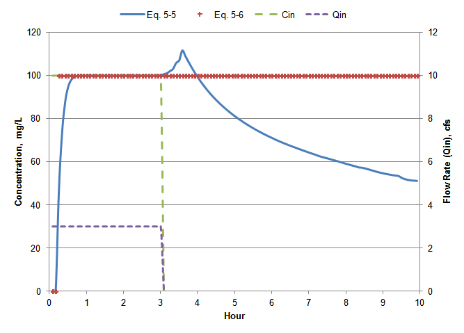
Figure 5‑3 Comparison of completely mixed reactor equations for a step inflow
Water quality routing computations are implemented as part of SWMM's conveyance system routing calculations. They are made at each flow routing time step immediately after a new set of flow rates and volumes has been computed for all elements of the conveyance network. Volume II of this manual describes in detail the procedures used for hydraulic routing.
The following quantities are therefore known for each pollutant and each network link:
*QL1(t+∆t)* = flow rate entering the link at time t+∆t (cfs)
*QL2(t+∆t)* = flow rate exiting the link at time t+∆t (cfs)
*VL(t)* = the volume of water stored in the link at time t (ft3)
*cL(t)* = the concentration of the pollutant in the link at time t (mass/ft3)
In addition, the following quantities are known for each pollutant at each node of the network at time t:
*VN(t)* = the volume of water stored at the node (ft3)
*cN(t)* = the concentration of the pollutant at the node at time t (mass/ft3)
Note that for computational purposes, concentration is expressed as mass/ft3. After computations are completed, they are converted back to mass/L for reporting purposes. The objective is to compute values of *cL* for each link and *cN* for each node at time t+∆t.
Using Equation 5-6 as its mixing equation for both conduit links and storage nodes, SWMM 5 carries out the following three step process to update pollutant concentrations for each node and link in the conveyance network at the end of each flow routing time step:
Certain modifications must be made to this basic procedure to handle the following special conditions.
Evaporation Losses
Both open conduits and storage units can lose water through evaporation. When water is evaporated, the pollutant mass stays behind (unless it volatilizes, which is not explicitly modeled by SWMM, although it could be approximated through the first order decay process). Thus when evaporation occurs pollutant concentrations will increase. SWMM computes this increase as a multiplier \(f_{evap}\):
\[f_{evap} = 1 + V_{evap}(t)/V(t)\]
(5-7)
where \(V_{evap}(t)\) is the volume lost to evaporation over the time step and \(V(t)\) is either *VN(t)* for a storage node at Step 2 or *VL(t)* for a conduit link at Step 3. This multiplier is then used to adjust the concentration *cN(t)* before Step 2 is carried out for a storage node or *cL(t)* before Step 3 is carried out for a conduit link.
Dynamic Wave Flow Routing
When SWMM's Dynamic Wave flow routing option (see Volume II) is used there is only one flow rate associated with each conduit, so that *QL1* and *QL2* have the same values. This might suggest that there would be no volume change within the conduit over a time step. However the routing process actually does produce a change in volume due to changes in flow depths at either end of the conduit. To make the flow rates consistent with this volume change, the value of *QL1* is adjusted by an amount ∆ \(Q_{L1}\) found from the following flow balance equation:
\[\mathrm{\Delta}Q_{L1} = V_{L}(t + \mathrm{\Delta}t) + V_{losses}(t) - V_{L}(t)\]
(5-8)
where \(V_{losses}(t)\) is the volume of evaporation and seepage loss over the time period \(\mathrm{\Delta}t\).
Steady Flow Routing
SWMM's Steady Flow routing option (see Volume II) simply translates the inflow to a conduit instantaneously to its outlet node. That is, the inflow to the conduit completely replaces the previous contents over the time step. So there is no mixing of the previous contents with new inflow from the upstream node. Thus Step 3 of the basic water quality routing procedure becomes:
\[c_{L}(t + \mathrm{\Delta}t) = f_{evap}c_{N}(t + \mathrm{\Delta}t)exp( - K_{1}\mathrm{\Delta}t)\]
(5-9)
where \(c_{N}(t + \mathrm{\Delta}t)\) is the newly computed concentration at the conduit's upstream node.
Management of stormwater quality is usually performed through a combination of so-called "best management practices" (BMPs) and a form of hydrologic source control popularly known as "low impact development" (LID). Treatment of stormwater runoff, either by natural means or by engineered devices, can occur at both the source of the generated runoff or at locations within the conveyance network. Source treatment through LID is discussed in the next chapter. This section describes how SWMM models treatment applied to flows already captured and transported within a conveyance system.
Table 5-1, adapted from Huber et al. (2006), categorizes the different unit treatment processes used by various types of conveyance system BMPs. Ideally one would like to model these processes at a fundamental level, to be able to estimate pollutant removal based on physical design parameters, hydraulic variables, and intrinsic chemical properties and reaction rates. With a few exceptions, the state of our knowledge does not permit this, at least within the scope of a general purpose stormwater management model like SWMM. Instead one has to rely on empirical relationships developed from site-specific monitoring data.
Strecker et al. (2001) discuss the challenges of using monitoring data to develop consistent estimates of BMP effectiveness and pollutant removal. The International Stormwater BMP Database (www.bmpdatabase.org) provides a comprehensive compilation of BMP performance data from over 500 BMP studies on 17 different categories of BMPs and LID practices. It is continually updated with new data contributed by the stormwater management community. Table 5-2 lists the median influent and effluent event mean concentrations (EMCs) for a variety of BMP categories and pollutants that were compiled from this database. The cells highlighted in yellow indicate that a statistically significant removal of the pollutant was achieved by the BMP category. A summary of the median removal percentages of several common pollutants treated by filtration, ponds, and wetlands published in the Minnesota Stormwater Manual is listed in Table 5-3. Most of these percentages are consistent with those inferred from median EMC numbers in the BMP database table 5-2.
Table 5‑1 Treatment processes used by various types of BMPs
| Process | Definition | Example BMPs |
|---|---|---|
| Sedimentation | Gravitational settling of suspended particles from the water column. | Ponds, wetlands, vaults, and tanks. |
| Flotation | Separation of particulates with a specific gravity less than water (e.g., trash, oil and grease). | Oil-water separators, density separators, dissolved-air flotation. |
| Filtration | Removal of particulates by passing water through a porous medium like sand, gravel, soil, etc. | Sand filters, screens, and bar racks. |
| Infiltration | Allowing captured runoff to infiltrate into the ground reducing both runoff volume and loadings of particulates and dissolved nutrients and heavy metals. | Infiltration basins, ponds, and constructed wetlands. |
| Adsorption | Binding of contaminants to clay particles, vegetation or certain filter media. | Infiltration systems, sand filters with iron oxide, constructed wetlands. |
| Biological Uptake and Conversion | Uptake of nutrients by aquatic plants and microorganisms; conversion of organics to less harmful compounds by bacteria and other organisms. | Ponds and wetlands. |
| Chemical Treatment | Chemicals used to promote settling and filtration. Disinfectants used to treat combined sewer overflows. | Ponds, wetlands, rapid mixing devices. |
| Natural Degradation (volatilization, hydrolysis, photolysis) | Chemical decomposition or conversion to a gaseous state by natural processes. | Ponds and wetlands. |
| Hydrodynamic Separation | Uses the physics of flowing water to create a swirling vortex to remove both settleable particulates and flotables. | Swirl concentrators, secondary current devices, oil-water separators. |
Table 5‑2 Median inlet and outlet EMCs for selected stormwater treatment practices
| Pollutant | Media Filtration | Detention Basin | Retention Pond | Wetland Basin | Manufactured Device | |||||
|---|---|---|---|---|---|---|---|---|---|---|
| In | Out | In | Out | In | Out | In | Out | In | Out | |
| TSS mg/L | 52.7 | 8.7 | 66.8 | 24.2 | 70.7 | 13.5 | 20.4 | 9.06 | 34.5 | 18.4 |
| F. Coliform, #/100mL | 1350 | 542 | 1480 | 1030 | 1920 | 707 | 13000 | 6140 | 2210 | 2750 |
| Cadmium, ug/L | 0.31 | 0.16 | 0.39 | 0.31 | 0.49 | 0.23 | 0.31 | 0.18 | 0.40 | 0.28 |
| Chromium, ug/L | 2.02 | 1.02 | 5.02 | 2.97 | 4.09 | 1.36 | 3.66 | 2.82 | ||
| Copper, ug/L | 11.28 | 6.01 | 10.62 | 5.67 | 9.57 | 4.99 | 5.61 | 3.57 | 13.42 | 10.16 |
| Lead, ug/L | 10.5 | 1.69 | 6.08 | 3.10 | 8.48 | 2.76 | 2.03 | 1.21 | 8.24 | 4.63 |
| Nickel, ug/L | 3.51 | 2.20 | 5.64 | 3.35 | 4.46 | 2.19 | 3.84 | 4.51 | ||
| Zinc, ug/L | 77.3 | 17.9 | 70.0 | 17.9 | 53.6 | 21.2 | 48.0 | 22.0 | 87.7 | 58.5 |
| Total P, mg/L | 0.18 | 0.09 | 0.28 | 0.22 | 0.30 | 0.13 | 0.13 | 0.08 | 0.19 | 0.12 |
| Orthophosphate, mg/L | 0.05 | 0.03 | 0.53 | 0.39 | 0.10 | 0.04 | 0.04 | 0.02 | 0.21 | 0.10 |
| Total N, mg/L | 1.06 | 0.82 | 1.40 | 2.37 | 1.83 | 1.28 | 1.14 | 1.19 | 2.27 | 2.22 |
| TKN, mg/L | 0.96 | 0.57 | 1.49 | 1.61 | 1.28 | 1.05 | 0.95 | 1.01 | 1.59 | 1.48 |
| NOX, mg/L | 0.33 | 0.51 | 0.55 | 0.36 | 0.43 | 0.18 | 0.24 | 0.08 | 0.41 | 0.41 |
Source: International Stormwater BMP Database, "International Stormwater Best Management Practices (BMP) Database Pollutant Category Summary Statistical Addendum: TSS, Bacteria, Nutrients, and Metals", July 2012 (www.bmpdatabase.org).
Table 5‑3 Median pollutant removal percentages for select stormwater BMPs
| Pollutant | Sand Filter | Ponds | Wetlands |
|---|---|---|---|
| Total Suspended Solids | 85 | 84 | 73 |
| Total Phosphorus | 77 | 50 | 38 |
| Particulate Phosphorus | 91 | 91 | 69 |
| Dissolved Phosphorus | 60 | 0 | 0 |
| Total Nitrogen | 35 | 30 | 30 |
| Zinc and Copper | 50 | 70 | 70 |
| Bacteria | 80 | 60 | 60 |
Source: Minnesota Stormwater Manual (http://stormwater.pca.state.mn.us).
SWMM 5 allows treatment to be applied to any water quality constituent at any node of the conveyance network. Treatment will act to reduce the nodal concentration of the constituent from the value it had after Step 2 of the water quality routing procedure described in section 5.3 (after a new mixture concentration has been computed for the node but before any outflow from the node is sent into any downstream links). The degree of treatment for a constituent is prescribed by the user, either as a concentration remaining after treatment or as the fractional removal achieved. It can be a function of the current concentration or fractional removal of any set of constituents as well as the current flow rate. For storage nodes, it can also depend on water depth, surface area, routing time step, and hydraulic residence time. Because treatment is applied at every time step, the resulting pollutant concentrations can vary throughout a storm event and will not necessarily represent an event mean concentration (EMC). The exception, of course, would be if treatment is specified as simply a constant concentration that is not dependent on any other variables.
The effect of treatment for a particular pollutant at a particular node can be expressed mathematically using one of the following general expressions (some specific examples will be presented later on):
\[c(t + \mathrm{\Delta}t) = c(\mathbf{C},\ \mathbf{R},\ \mathbf{H})\ \]
(5-10)
\[c(t + \mathrm{\Delta}t) = \left( 1 - r\left( \mathbf{C},\ \mathbf{R},\ \mathbf{H} \right) \right)C_{in}(t + \mathrm{\Delta}t)\ \]
(5-11)
where:
\(c\) = nodal pollutant concentration after treatment is applied
\(C_{in}\) = pollutant concentration in the node's inflow stream
\(c(\ldots)\) = concentration-based treatment function
\(r(\ldots)\) = removal-based treatment function
\(\mathbf{C}\) = vector of nodal pollutant concentrations before treatment is applied
\(\mathbf{C}_{\mathbf{in}}\) = vector of pollutant concentrations in the node's inflow stream
\(\mathbf{R}\) = vector of fractional removals resulting from treatment
\(\mathbf{H}\) = vector of hydraulic variables at the current time step.
Note that if treatment is made a function of pollutant concentrations, then for concentration-based treatment these represent the concentrations at the node prior to treatment while for removal-based functions they are the concentrations in the node's combined influent stream. If the node has no volume (e.g., is a non-storage node) then these two types of concentrations are equivalent.
The hydraulic variables that can appear in a treatment expression include the following:
FLOW flow rate into the node in user defined flow units
DEPTH average water depth in the node over the time step (ft or m)
AREA average surface area of the node over the time step (ft2 or m2)
DT current routing time step (seconds)
HRT hydraulic residence time of water in a storage node (hours).
The hydraulic residence time is the average time that water has spent within a completely mixed storage node. It is continuously updated for each storage node as the simulation progresses by evaluating the following expression:
\[\theta(t + \mathrm{\Delta}t) = (\theta(t) + \mathrm{\Delta}t)\frac{V(t)}{V(t) + Q_{in}\mathrm{\Delta}t}\ \]
(5-12)
where \(\theta(t)\) is the hydraulic residence time at time t in seconds, \(V(t)\) is the cubic feet of stored water at time t, \(Q_{in}\) is the inflow rate to the storage node in cfs, and \(\mathrm{\Delta}t\) is the current time step in seconds.
SWMM applies the following conditions when evaluating a treatment expression:
The latter condition is necessary because co-pollutants only apply to buildup/washoff processes – not to the user-specified concentrations in rainwater, groundwater, I/I, dry weather flow, and externally imposed inflows.
Several concrete examples of treatment expressions, in the format used by SWMM 5's input file, will be given to illustrate how different types of treatment mechanisms can be modeled.
EMC Treatment
Treatment results in a constant concentration. As an example, if this concentration were 10 mg/L then the treatment expression supplied to SWMM would be:
c = 10
Constant Removal Treatment
Treatment results in a constant percent removal. For example, if this removal was 85% then the treatment expression would be:
r = 0.85
Co-Removal Treatment
The removal of some pollutant is proportional to the removal of some other pollutant. For example, if the removal of pollutant X was 75% of the removal of suspended solids (TSS) then the treatment expression would be:
r = 0.75 * R_TSS
where R_TSS is the fractional removal computed for pollutant TSS.
Concentration-Dependent Removal
Some empirical performance data indicate higher pollutant removal efficiencies with higher influent concentrations (Strecker et al., 2001). Suppose that the removal of pollutant X is 50% for inflow concentrations below 50 mg/L and 75% for concentrations above 50. The resulting treatment expression would be:
r = (1 - STEP(C_X – 50)) * 0.5 + STEP(C_X – 50) * 0.75
where C_X is the influent concentration of pollutant X and STEP is the unit step function whose value is zero for negative argument and one for positive argument.
N-th Order Reaction Kinetics
Suppose that during treatment pollutant X exhibits n-th order reaction kinetics where the instantaneous reaction rate is \(kC^{n}\) with k being the rate constant and n the reaction order. This can be represented as the following SWMM treatment expression for the specific case where k = 0.02 and n = 1.5:
c = C_X – 0.02 * (C_X\^1.5) * DT
The k-C* Model
This is a first-order model with background concentration made popular by Kadlec and Knight (1996) for long-term treatment performance of wetlands. The general model can be expressed as:
\[c - C^{*} = \left( C_{in} - C^{*} \right)exp( - \frac{k\theta}{d})\]
(5-13)
where \(C^{*}\) is a constant residual concentration that always remains, k is a rate coefficient with units of length/time, θ is the hydraulic residence time, and d is water depth. This equation can be re-arranged into a removal function as follows:
\[r = 1 - \frac{c}{C_{in}} = \left\lbrack 1 - \exp\left( - \frac{k\theta}{d} \right) \right\rbrack\left\lbrack 1 - \frac{C^{*}}{C_{in}} \right\rbrack\]
(5-14)
The corresponding SWMM removal expression of some pollutant X with k = 0.02 (ft/hr) and \(C^{*}\) = 20 would look as follows:
r = STEP(C_X – 20) * ((1 – exp(-0.02*HRT/DEPTH)) * (1-20/C_X))
The STEP(C_X – 20) term insures that no removal occurs when the inflow concentration is below the residual concentration.
Gravity Settling
Consider a size range of suspended particles with average settling velocity *ui. During a quiescent period of time *∆t within a storage volume the fraction of these particles that will settle out is \(u_{i}\mathrm{\Delta}t/d\) where d is the water depth. Summing over all particle size ranges leads to the following expression for the change in TSS concentration ΔC during a time step Δt:
\[\mathrm{\Delta}c = c(t)\sum_{i}^{}{f_{i}u_{i}}\left( \frac{\mathrm{\Delta}t}{d} \right)\]
(5-15)
where \(f_{i}\) is the fraction of particles with settling velocity \(u_{i}\). Because \(\sum_{}^{}{f_{i}u_{i}}\) is generally not known, it can be replaced with a fitting parameter k and in the limit Equation 5-15 becomes:
\[\frac{\partial c}{\partial t} = - \frac{k}{d}c(t)\]
(5-16)
Note that k has units of velocity (length/time) and can be thought of as a representative settling velocity for the particles that make up the total suspended solids in solution. Integrating 5-16 between times t and t + ∆t, and assuming there is some residual amount of suspended solids C* that is non-settleable leads to the following expression for \(c(t + \mathrm{\Delta}t)\):
\[c(t + \mathrm{\Delta}t) = C^{*} + \left( c(t) - C^{*} \right)exp( - \frac{k\mathrm{\Delta}t}{d})\]
(5-17)
For particular values of C* = 20 and k = 0.01 ft/hr this equation would be represented by the following treatment expression for a pollutant named TSS:
C = STEP(0.1 - FLOW) *
(20 + (C_TSS – 20) * exp(-0.01/DEPTH*DT/3600)) +
(1 – STEP(0.1 - FLOW)) * C_TSS
Note that DT is converted from seconds to hours to be compatible with the time units of k and that the STEP function is used to define quiescent conditions by an inflow rate below 0.1 cfs.
Figure 5.4 shows the result of using this treatment expression when routing a 6-hour runoff hydrograph with a peak flow of 20 cfs through a half acre dry detention pond whose outlet is a 9" high by 18" wide orifice. The TSS in the runoff has a constant EMC of 100 mg/L. The resulting TSS concentration in the pond over both the filling and emptying periods are plotted in the figure, as are the inflow hydrograph and pond water depth. Note that during the inflow period the TSS remains at 100 mg/L and begins to settle out once the inflow ceases. As the pond depth decreases while it empties more solids settle out reducing the TSS level until the residual concentration of 20 mg/L is reached.
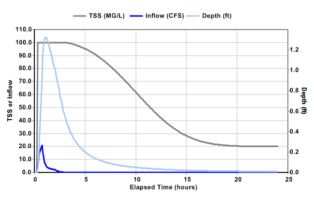
Figure 5‑4 Gravity settling treatment of TSS within a detention pond
The modern OpenSWMM engine implements the treatment system described above with a compiled expression language. Each treatment expression supplied in the input file's [TREATMENT] section has the form:
R = <expression> or C = <expression>
where the left hand side must be exactly R (the expression computes a fractional removal, Equation 5-11) or C (the expression computes a treated concentration, Equation 5-10). Each expression is parsed once at simulation initialization into a postfix token list (using the shunting-yard algorithm) and is evaluated with a stack machine at every routing time step, so expression complexity adds no per-step parsing cost.
The right hand side may contain numeric constants (including scientific notation), parentheses, the arithmetic operators + - * / ^ (with standard precedence and a unary minus), and the variables and functions listed in Tables 5-4 and 5-5. Variable and function names are case-insensitive.
Table 5‑4 Variables available in treatment expressions
| Variable | Meaning | Units |
|---|---|---|
| C | Pollutant concentration — the inflow concentration *Cin* in an R = expression, or the nodal concentration prior to treatment in a C = expression | concentration units |
| Q | Flow rate into the node (legacy SWMM 5 name FLOW) | user flow units |
| D | Average water depth in the node over the time step (legacy SWMM 5 name DEPTH) | ft or m |
| AREA | Average node surface area over the time step | ft2 or m2 |
| V | Volume of water stored at the node | ft3 |
| DT | Current routing time step | seconds |
| HRT | Hydraulic residence time of a storage node (Equation 5-12) | hours |
Note that the modern engine uses the short names Q and D in place of the legacy SWMM 5 names FLOW and DEPTH that appear in the examples of Section 5.4.3, and adds the stored volume V as an additional process variable. Co-pollutant references of the form C_pollutant and R_pollutant, used by the Co-Removal and Concentration-Dependent examples of Section 5.4.3, are part of the legacy SWMM 5 expression language; they are recognized by the modern expression grammar but are not currently compiled by the engine, and the expression validator reports them as unsupported.
Table 5‑5 Math functions available in treatment expressions
| Function | Meaning |
|---|---|
| exp(x) | Exponential ex |
| log(x), ln(x) | Natural logarithm (evaluates to 0 when x ≤ 0) |
| sqrt(x) | Square root (evaluates to 0 when x < 0) |
| abs(x) | Absolute value |
| sgn(x) | Sign function (-1, 0, or +1) |
| step(x) | Unit step function (1 when x > 0, otherwise 0) |
| min(x, y) | Smaller of the two arguments |
| max(x, y) | Larger of the two arguments |
Evaluation is guarded so that a treatment expression can never produce a non-finite result: division by zero evaluates to 0, as do the logarithm of a non-positive argument and the square root of a negative argument. After evaluation the result is clamped exactly as described in Section 5.4.2 — a fractional removal is limited to the range [0, 1] and a treated concentration is limited to the range from 0 up to the concentration prior to treatment.
Treatment is applied at each node immediately after the mixed nodal concentration has been computed (Step 2 of Section 5.3) and before any first-order decay. As part of this step the hydraulic residence time of each storage node with treatment is updated using Equation 5-12. The pollutant mass removed by treatment is accumulated into the water quality mass balance as reacted mass, so treated mass appears in the continuity report alongside first-order decay losses.
Treatment expressions can also be inspected and edited at run time through the programmatic C API. swmm_treatment_set, swmm_treatment_get, and swmm_treatment_clear read or replace the expression assigned to a (node, pollutant) pair; a mid-run edit is recompiled immediately and takes effect at the next quality routing step. The companion function swmm_treatment_validate_expression checks an expression against the production grammar without modifying any engine state, returning a human-readable diagnostic message and the character position of the first error. It is intended for editor and GUI use (e.g., validating an expression on every keystroke) and is deliberately stricter than the runtime tokenizer in one respect: characters that the tokenizer would silently skip are reported as errors. See openswmm_quality.h for the full API.
Implementation notes: The expression parser and stack-machine evaluator reside in src/engine/quality/Treatment.cpp (namespace openswmm::treatment). Treatment application, HRT updating, and mass-balance accounting are implemented in QualitySolver::applyTreatment() in src/engine/quality/QualityRouting.cpp. Expressions are compiled during quality initialization in src/engine/core/SWMMEngine.cpp, and the C API entry points are declared in openswmm_quality.h.
[OPTIONS] QUALITY_SOLVER and share this chapter's external loads, treatment expressions and mass-balance ledger.  1.13.2