3.1 Introduction

Simulation of pollutant buildup on the subcatchment surface is only required if SWMM's Exponential option is used to describe wash off, since that function depends on the amount of buildup present (see Chapter 4). However, even when washoff quality is estimated using an Event Mean Concentration (EMC) or Rating Curve option, buildup simulation could still be useful to establish a maximum mass of pollutant that could be removed during any given storm event.

One of the most influential of the early studies of stormwater pollution was conducted in Chicago by the American Public Works Association (1969). As part of this project, street surface accumulation of "dust and dirt" (DD) (anything passing through a quarter-inch mesh screen) was measured by sweeping with brooms and vacuum cleaners. The accumulations were measured for different land uses and curb length, and the data were normalized in terms of pounds of dust and dirt per dry day per 100 ft of curb or gutter. These well known results are shown in Table 3-1 and imply that dust and dirt buildup is a linear function of time. The dust and dirt samples were analyzed chemically, and the fraction of sample consisting of various constituents for each of four land uses was determined, leading to the results shown in Table 3-2.

Table 3-1 Measured dust and dirt (DD) accumulation in Chicago Source: APWA (1969).

Type	Land Use	Pounds DD/dry day per 100 ft-curb
1	Single Family Residential	0.7
2	Multi-Family Residential	2.3
3	Commercial	3.3
4	Industrial	4.6
5	Undeveloped or Park	1.5

Table 3-2 Milligrams of pollutant per gram of dust and dirt (parts per thousand by mass) for four Chicago land uses Source: APWA (1969).

Parameter	Single Family Residential	Multi-Family Residential	Commercial	Industrial
BOD5	5.0	3.6	7.7	3.0
COD	40.0	40.0	39.0	40.0
Total Coliforms^a	1.3 × 10⁶	2.7 × 10⁶	1.7 × 10⁶	1.0 × 10⁶
Total N	0.48	0.61	0.41	0.43
Total PO₄ (as PO₄)	0.05	0.05	0.07	0.03

^aUnits for coliforms are MPN/gram.

From the values shown in Tables 3-1 and 3-2, the buildup of each constituent (also linear with time) can be computed simply by multiplying dust and dirt by the appropriate fraction. Since the APWA study was published during the original SWMM project (1968-1971), it represented the state of the art at the time and linear buildup was used extensively in the development of the surface quality routines in the original SWMM program (Metcalf and Eddy et al., 1971a, Section 11). Ammon (1979) summarized many subsequent studies of pollutant buildup on urban surfaces and found evidence to suggest several nonlinear buildup relationships as alternatives to the linear one. Upper limits for buildup are also likely. Several options for both buildup and washoff were proposed by Ammon and incorporated into SWMM III (Huber et al., 1981b).

Of course, the whole buildup idea essentially ignores the physics of generation of pollutants from sources such as street pavement, vehicles, atmospheric fallout, vegetation, land surfaces, litter, spills, anti-skid compounds and chemicals, construction, and drainage networks. Novotny and Olem (1994) and Novotny (1995) summarize empirical relationships for the urban street surface pollution accumulation process. Lager et al. (1977) and James and Boregowda (1985) consider each source in turn and give guidance on buildup rates. To summarize, several studies and voluminous data exist from the 1960s and 1970s with which to formulate buildup relationships, most of which are purely empirical and data-based, ignoring the underlying physics and chemistry of the generation processes. Nonetheless, they represent what is available, and modeling techniques in SWMM are designed to accommodate them in their heuristic form.

3.2 Governing Equations

There is ample evidence that buildup is a nonlinear function of dry days; Sartor and Boyd's (1972) data are most often cited as examples (Figure 3-1). Later data from Pitt (Figure 3-2) for San Jose indicate almost linear accumulation, although some of the best fit lines indicated in the figure had very poor correlation coefficients, ranging from 0.35 ≤ R ≤ 0.9. (The actual data points are not shown in Pitt's figures.) Even in data collected as carefully as in the San Jose study, the scatter (not shown in the report) is considerable. Thus, the choice of the best functional form is not obvious.

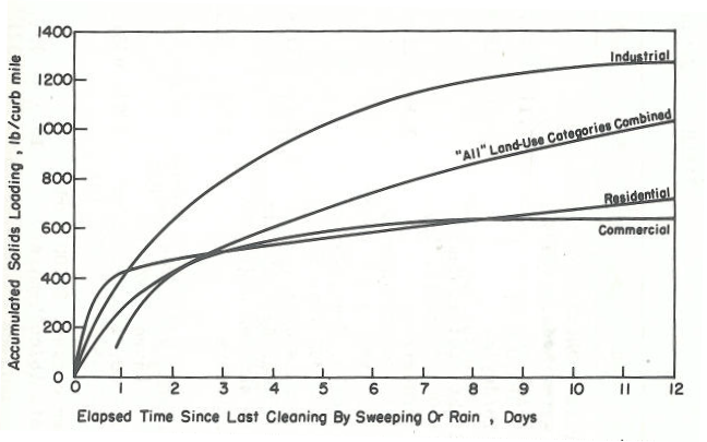
Figure 3‑1 Accumulation of solids on urban streets versus time (Sartor and Boyd, 1972)

Because buildup data clearly show that different rates apply to different land uses, SWMM allows one to define a different buildup function for each combination of pollutant and land use. The Pollutant object used to describe water quality constituents was described previously in section 2.3. SWMM's Land Use object is used to identify a particular type of land use and to store the buildup (and washoff) functions for each SWMM Pollutant.

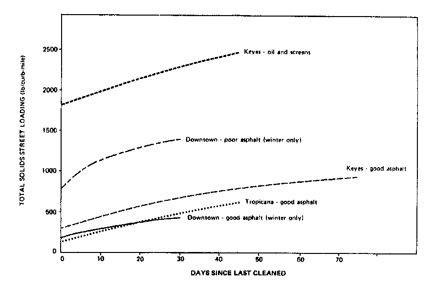
Figure 3‑2 Buildup of street solids in San Jose (from Pitt, 1979)

The buildup of each pollutant that accumulates over a category of land use is described by either a mass per unit of subcatchment area or per unit of curb length. For microbial constituents, numbers of organisms is used instead of mass. The choice of quantity to normalize against (area or curb length) can vary by pollutant and land use. In the discussion that follows [B] will denote the units being used to express buildup.

Because there is no obviously proper functional form that describes pollutant buildup over time, SWMM provides the user with three different functional options for any combination of constituent and land use. These are:

power function (of which linear buildup is a special case),
exponential, or
saturation.

Power function buildup accumulates proportional to time raised to some power, until a maximum limit is achieved,

\[b = Min(B_{\max},\ K_{B}t^{N_{B}})\]

(3-1a)

where

b = buildup, [B]

t = buildup time interval, days

*B_max* = maximum buildup possible, [B]

*K_B* = buildup rate constant, [B]-days^{-*N*^}_B*

*N_B* = buildup time exponent, dimensionless

The time exponent, *N_B,* should be ≤ 1 so that a decreasing rate of buildup occurs as time increases. When *N_B* is set equal to 1, a linear buildup function is obtained.

Exponential buildup follows an exponential growth curve that approaches a maximum limit asymptotically,

\[b = B_{\max}\left( 1 - e^{- K_{B}t} \right)\]

(3-1b)

where the rate constant *K_B* now has units of days^-1.

Saturation buildup begins at a linear rate which proceeds to decline constantly over time until a saturation value is reached,

\[b = \frac{B_{\max}t}{\left( K_{B} + t \right)}\]

(3-1c)

where now *K_B* is a half saturation constant (days to reach half of the maximum buildup).

Table 3-3 summarizes the meaning and units of the coefficients used in each of the buildup functions. The following expression will convert from mass of buildup per unit of area or curb length for a specific land use to total mass

\[m_{B} = bNf_{LU}\]

where *m_B* = mass of buildup, b = mass per unit of either area or curb length, N = total area or curb length for the subcatchment in question, and *f_LU* = fraction of the subcatchment's area devoted to the land use in question.

The shapes of the three functions are compared in Figure 3-3 using a hypothetical pollutant as an example that reaches a maximum buildup of 2 kg/ac in about 14 days. The Exponential and Saturation functions have clearly defined asymptotes or upper limits (2 kg/ac in this figure). Upper limits for linear or power function buildup may be imposed if desired. "Instantaneous buildup" may be easily achieved using the power function with *N_B* set to 0 and *K_B* set equal to *B_max*. This would result in a constant buildup of *B_max* which would always be available at the beginning of any storm event.

Table 3-3 Summary of buildup function coefficients

Coefficient	Power	Exponential	Saturation
Bmax	buildup limit [B]	buildup limit [B]	buildup limit [B]
K_B	rate constant, [B]days^{-N^}_B*	rate constant, days^-1	½ saturation constant, days
N_B	time exponent

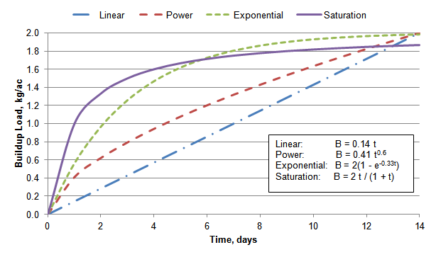
Figure 3‑3 Comparison of buildup equations for a hypothetical pollutant

It is apparent from Figure 3-3 that different options may be used to accomplish the same objective (e.g., nonlinear buildup); the choice may well be made on the basis of available data to which one of the functional forms has been fit. If an asymptotic form is desired, either the exponential or saturation option may be used depending upon ease of comprehension of the parameters. For instance, for exponential buildup the rate constant, *K_B*, is the familiar exponential decay constant. It may be obtained from the slope of a semi-log plot of buildup versus time. As a numerical example, if its value were 0.33 day^‑1, then it would take 7 days to reach 90 percent of the maximum buildup, as in Figure 3-3.

For saturation buildup the parameter *K_B* has the interpretation of the half saturation constant, that is, the time at which buildup is half of the maximum (asymptotic) value. For instance, the *K_B* of 1 day for the saturation curve in Figure 3-3 corresponds to the time where the buildup reaches half the maximum amount. If the asymptotic value *B_max* is known or estimated, K*_B* may be obtained from buildup data from the slope of a plot of b versus t × (*B_max* - b). Generally, the saturation formulation will rise steeply (in fact, linearly for small t) and then approach the asymptote slowly.

The power function may be easily adjusted to resemble asymptotic behavior, but it must always ultimately exceed the maximum value (if used). The parameters are readily found from a log-log plot of buildup versus time. This is a common way of analyzing data, (e.g., Miller et al., 1978; Ammon, 1979; Smolenyak, 1979; Jewell et al., 1980; Wallace, 1980).

When applying a buildup function in dry periods in conjunction with a washoff function in wet periods it is useful to know the number of days t it takes to reach a given amount of buildup b. This can be found by re-arranging Equation 3-1 as follows:

\(t = \left( \frac{b}{K_{B}} \right)^{\frac{1}{N_{B}}}\) for power buildup (3-2a)

\(t = \frac{- ln\left( 1 - \frac{b}{B_{\max}} \right)}{K_{B}}\) for exponential buildup
(3-2b)

\(t = \frac{bK_{B}}{\left( B_{\max} - b \right)}\) for saturation buildup (3-2c)

Note that when *N_B = 0* for power buildup then buildup b is a constant value *B_max* for all times t. Figure 3-4 shows how buildup is adjusted between and after storm events. Assume that b*0* represents the amount of buildup present at the start of a storm event. The event washes off part of that buildup leaving an amount b1 remaining. Equation 3-2 is used to find the time t1 associated with buildup b1. If a dry period of length ∆t occurs before the start of the next storm, then the amount of buildup available, b2, is found by evaluating the buildup function at time t2 = t1 + ∆t.

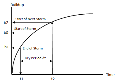
Figure 3‑4 Evolution of buildup after a storm event

3.3 Computational Steps

Pollutant buildup computations are a sub-procedure implemented as part of SWMM's runoff calculations. They are made at each runoff time step for each subcatchment immediately after surface runoff has been computed as described in Section 3.4 of Volume I. The following constant quantities are known for each subcatchment:

A (the subcatchment area),
L (the curb length of streets in the subcatchment (if used to normalize buildup)),
*f_LU* ( the fraction of the subcatchment's area devoted to a particular land use,
*B_max*, *K_B,* and *N_B* for each combination of pollutant and land use.

Note that a pollutant's buildup constants vary by land use, not by subcatchment. That is, if residential land is assigned a set of buildup constants then those constants apply to the residential portion of all subcatchments. Also available is the buildup *m_B* (in mass units) for each pollutant on each land use in the subcatchment at the start of the current time period. Initially at time zero, *m_B* is established in one of two ways:

If the user specified an initial buildup (as mass per area) of the pollutant over the entire subcatchment, then the initial *m_B* equals that buildup times the area devoted to the particular land use.
Otherwise a user-supplied antecedent dry days value is used with Equation 3-1 to determine an initial buildup per area (or curb length) with the result multiplied by the area (or curb length) associated with the land use to obtain an initial mass *m_B*.

The computational steps for updating the buildup of a specific pollutant - land use combination within a subcatchment over a single time step are:

If the runoff rate is greater than 0.001 in/hr then the time step is assumed to belong to a wet weather event and no buildup addition occurs (buildup will actually be reduced according to the amount of washoff produced as described later in Chapter 4).
If buildup for the pollutant has been designated to occur only when snow is present and the current snow depth is less than 0.001 inches then no buildup addition occurs.
Convert the total mass of buildup *m_B* to a normalized mass b by dividing it by \(f_{LU}A\) if buildup is normalized with respect to area or \(f_{LU}L\) if normalized with respect to curb length.
Use Equation 3-2 to find the time t corresponding to normalized buildup b.
Add the length of the current runoff time step to t and use this value in Equation 3-1 to find an updated value for b.
Convert the new normalized buildup b back to total mass *m_B* by multiplying it by the normalizing factor (either \(f_{LU}A\) or \(f_{LU}L\)).

This process will produce a new set of pollutant mass buildups *m_B* at the end of the runoff time step for each land use within each subcatchment. These buildups will then be used to compute washoff loads (as described in Section 4) when the next wet period occurs.

3.4 Street Cleaning

Street cleaning is performed in most urban areas for control of solids and trash deposited along street gutters. Although it has long been assumed that street cleaning has a beneficial effect upon the quality of urban runoff, until recently, few data have been available to quantify this effect. Unless performed on a daily basis, EPA Nationwide Urban Runoff Program (NURP) studies generally found little improvement of runoff quality by street cleaning (EPA, 1983b). On the other hand, more recent studies indicate that technological advances in cleaning equipment can produce much better results (Sutherland and Jelen, 1997).

The most elaborate studies are probably those of Pitt (1979, 1985) in which street surface loadings were carefully monitored along with runoff quality in order to determine the effectiveness of street cleaning. In San Jose, California Pitt (1979) found that frequent street cleaning on smooth asphalt surfaces (once or twice per day) can remove up to 50 percent of the total solids and heavy metal yields of urban runoff. Under more typical cleaning programs of once or twice a month, less than 5 percent of these contaminants were removed. Organics and nutrients in the runoff cannot be effectively controlled by intensive street cleaning – typically much less than 10 percent removal, even for daily cleaning. This is because the latter originate primarily in runoff and erosion from off-street areas during storms. In Bellevue, Washington, Pitt (1985) reached similar conclusions, with a maximum projected effectiveness for pollutant removal from runoff of about 10 percent.

The removal effectiveness of street cleaning depends upon many factors such as the type of sweeper, whether flushing is included, the presence of parked cars, the quantity of total solids, the constituent being considered, and the relative frequency of rainfall events. Obviously, if street sweeping is performed infrequently in relation to rainfall events, it will not be effective. Removal efficiencies for several constituents are shown in Table 3-4 (Pitt, 1979). Clearly, efficiencies are greater for constituents that behave as particulates.

SWMM allows pollutant buildup within a given land use area to be reduced by street sweeping operations. This reduction is accounted for by having the user supply the following set of parameters:

*SS₁* = month/day of the year when street sweeping operations start

*SS₂* = month/day of the year when street sweeping operations end

SSI = number of days between street sweeping for a given land use

SS0 = number of days since the land use was last swept at the start of the simulation

SSA = fraction of buildup on the land use that is available for removal by sweeping

SSE = fraction of the available buildup of a pollutant on a given land use that is removed by sweeping

The availability factor, SSA, is intended to account for the fraction of a land use's area that is actually "sweepable." A single set of *SS₁* and *SS₂* values is supplied for the entire study area, SSI, SS0, and SSA values are supplied for each land use category within the study area, and an SSE value is supplied for each combination of pollutant and land use category.

Table 3-4 Removal efficiencies from street cleaner path for various street cleaning programs (Pitt, 1979)

Vacuum Street Cleaner - 20-200 lb/curb mile total solids

Passes	Total Solids	BOD₅	COD	KN	PO₄	Pesticides	Cd	Sr	Cu	Ni	Cr	Zn	Mn	Pb	Fe
1 pass	31	24	16	26	8	33	23	27	30	37	34	34	37	40	40
2 passes	45	35	22	37	12	50	34	35	45	54	53	52	56	59	59
3 passes	53	41	27	45	14	59	40	48	52	63	60	59	65	70	68

Vacuum Street Cleaner - 200-1,000 lb/curb mile total solids

Passes	Total Solids	BOD₅	COD	KN	PO₄	Pesticides	Cd	Sr	Cu	Ni	Cr	Zn	Mn	Pb	Fe
1 pass	37	29	21	31	12	40	30	34	36	43	42	41	45	49	59
2 passes	51	42	29	46	17	59	43	48	49	59	60	59	63	68	68
3 passes	58	47	35	51	20	67	50	53	59	68	66	67	70	76	75

Vacuum Street Cleaner - 1,000-10,000 lb/curb mile total solids

Passes	Total Solids	BOD₅	COD	KN	PO₄	Pesticides	Cd	Sr	Cu	Ni	Cr	Zn	Mn	Pb	Fe
1 pass	48	38	33	43	20	57	45	44	49	55	53	55	58	62	63
2 passes	60	50	42	54	25	72	57	55	63	70	68	69	72	79	77
3 passes	63	52	44	57	26	75	60	58	66	73	72	73	76	83	82

Mechanical Street Cleaner - 180-1,800 lb/curb mile total solids

Passes	Total Solids	BOD₅	COD	KN	PO₄	Pesticides	Cd	Sr	Cu	Ni	Cr	Zn	Mn	Pb	Fe
1 pass	54	40	31	40	20	40	28	40	38	45	44	43	47	44	49
2 passes	75	58	48	58	35	60	45	59	58	65	64	64	64	65	71
3 passes	85	69	59	69	46	72	57	70	69	76	75	75	79	77	82

Other Cleaning Methods

Method	Total Solids	Other Pollutants
Flusher	30	(a)
Mechanical Street Cleaner followed by a Flusher	80	(b)

(a) 15-40 percent estimated
(b) 35-100 percent estimated

These removal values assume all the pollutants would lie within the cleaner path (0 to 8 ft. from the curb)

If the date of the current time step falls within *SS₁* and *SS₂* then the buildup *m_B* found from the previous steps of Section 3.3 (for a specific pollutant and land use) is modified as follows:

If the current rainfall is above 0.001 in/hr or there is more than 0.05 inches of snow on the plowable impervious area of the subcatchment or SSI was set to zero then no sweeping occurs.
If the time between the current date and the date when the land use was last swept is less than SSI then no sweeping occurs.
Otherwise set \(\ m_{B} = m_{B}(1 - SSA \bullet SSE)\) for each of the land uses's pollutants and set the date when the land use was last swept to the current date.

3.5 Parameter Estimates

There is no single choice of buildup function or parameter values (which are pollutant- and land use-specific) that can be applied universally. Although data from the literature can help determine representative estimates there is no substitute for field data collected for the site in question. The discussion that follows presents sources of buildup data from studies that were made mainly in the 1970's or earlier.

The previously mentioned 1969 APWA study (APWA, 1969) was followed by several more efforts, notably AVCO (1970) (reporting extensive data from Tulsa, Oklahoma), Sartor and Boyd (1972) (reporting a cross section of data from ten U.S. cities), and Shaheen (1975) (reporting data for highways in the Washington, DC area). Pitt and Amy (1973) followed the Sartor and Boyd (1972) study with an analysis of heavy metals on street surfaces from the same ten cities. Later, Pitt (1979) reported on extensive data gathered both on the street surface and in runoff for San Jose. A drawback of the earlier studies is that it is difficult to draw conclusions from them on the relationship between street surface accumulation and stormwater concentrations since the two were seldom measured simultaneously.

Amy et al. (1974) provide a summary of data available in 1974 while Lager et al. (1977) provide a similar summary as of 1977 without the extensive data tabulations given by Amy et al. Perhaps the most comprehensive summary of surface accumulation and pollutant fraction data is provided by Manning et al. (1977) in which the many problems and facets of sampling and measurements are also discussed. For instance, some data are obtained by sweeping, others by flushing; the particle size characteristics and degree of removal from the street surface differ for each method. Some results of Manning et al. (1977) will be presented later. Surface accumulation data may be gleaned, somewhat less directly, from references on loading functions that include McElroy et al. (1976), Heaney et al. (1977) and Huber et al. (1981a). Regrettably, there seem to be no studies since the 1970s in which pollutant accumulation has been measured directly.

Manning et al. (1977) have perhaps the best summary of linear buildup rates; these are presented in Table 3-5. It may be noted that dust and dirt buildup varies considerably among three different studies. Individual constituent buildup may be taken directly from values in the table or computed as a fraction of dust and dirt (simulated as a pollutant) using the "Co-pollutant and Co-fraction" option described subsequently. It is apparent that although a large number of constituents have been sampled, little distinction can be made on the basis of land uses for most of them.

As an example, suppose dust and dirt (DD) is to be simulated as a co-pollutant and values are taken for commercial land use and from the "All Data" row in Table 3-5. Since the data are given as lb · curb-mile^-1 · day^-1, linear buildup is assumed and for commercial land use DD buildup (average for all data) is 116 lb/(curb-mile – day). Converting from pounds to milligrams (453,592 mg/lb) and mile to 1000-ft (5.28 1000-ft/mi) yields *K_B* = 9.97 x 10⁶ mg/1000-ft-day in Equation 3-1a, and of course, *N_B* = 1. Constituent fractions are available from the table. For instance, BOD5 as a fraction of DD for commercial land use would be 7.19 mg/g (or 0.00719 as a SWMM Co-fraction), 0.06 mg/g for total phosphorus, 0.00002 mg/g for Hg, and 36,900 MPN/g for fecal coliforms (36.9 MPN/mg as a SWMM input co-fraction). Direct loading rates could be computed for each constituent as an alternative. For instance, for BOD5, the linear buildup rate would equal 9.97 x 10⁶ · 0.00719 = 3,800 mg / (1000-ft curb - day).

Table 4-19 on pp. 4-94, 4-95, 4-96.It must be stressed once again that the generalized buildup data of Table 3-5 are merely informational and are never a substitute for local sampling or even a calibration using measured concentrations. They may serve as a first trial value for a calibration, however. In this respect it is important to point out that the concentrations and loads computed by the SWMM buildup-washoff algorithms are usually linearly proportional to buildup rates. If twice the quantity is available at the beginning of a storm, the concentrations and loads will be usually be doubled. Calibration is probably easiest with linear buildup parameters, but it depends on the rate at which the limiting buildup, i.e., *B_max*, is approached. If the limiting value is reached during the interval between most storms, then calibration using it will also have almost a linear effect on concentrations and loads.

Table 3-5 Nationwide data on linear dust and dirt buildup rates and on pollutant fractions (after Manning et al., 1977)

Dust and Dirt Accumulation (kg/curb-km/day)

Study	Statistic	Single Family Residential	Multi-Family Residential	Commercial	Industrial	All Data
Chicago<sup>(1)	Mean	10	31	51	92	44
	Range	5-27	17-43	80-151	80-151	5-15
	N	60	93	126	55	334
Washington<sup>(2)	Mean	—	—	38	—	38
	Range	—	—	10-103	—	10-103
	N	—	—	22	—	22
Multi-City⁽³⁾	Mean	51	44	13	81	49
	Range	1-268	2-217	1-73	1-423	1-423
	N	14	8	10	12	44
All Data	Mean	17	32	47	90	45
	Range	1-268	2-217	1-103	1-423	1-423
	N	74	101	158	67	400

Pollutant Fractions

Pollutant	Statistic	Single Family Residential	Multi-Family Residential	Commercial	Industrial	All Data
BOD (g/kg)	Mean	5.26	3.37	7.19	2.92	5.03
	Range	1.72-9.43	2.03-6.32	1.28-14.54	2.82-2.95	1.29-14.54
	N	59	93	102	56	292
COD (g/kg)	Mean	39.25	41.97	61.73	25.08	46.12
	Range	18.30-72.80	24.6-61.3	24.8-498.41	23.0-31.8	18.3-498.41
	N	59	93	102	38	292
Total N-N (mg/kg)	Mean	460	550	420	430	480
	Range	325-525	356-961	323-480	410-431	323-480
	N	59	93	80	38	270
Kjeldahl N (mg/kg)	Mean	—	—	640	—	640
	Range	—	—	230-1,790	—	230-1,790
	N	—	—	22	—	22
NO₃ (mg/kg)	Mean	—	—	24	—	24
	Range	—	—	10-35	—	10-35
	N	—	—	21	—	21
NO₂-N (mg/kg)	Mean	—	—	0	—	15
	Range	—	—	0	—	0
	N	—	—	15	—	15
Total P (mg/kg)	Mean	—	—	170	—	170
	Range	—	—	90-340	—	90-340
	N	—	—	21	—	21
PO₄-P (mg/kg)	Mean	49	58	60	26	53
	Range	20-109	20-73	0-142	14-30	0-142
	N	59	93	101	38	291

Heavy Metals and Other Pollutants (mg/kg unless noted)

Pollutant	Statistic	Single Family Residential	Multi-Family Residential	Commercial	Industrial	All Data
Chlorides	Mean	—	—	220	—	220
	Range	—	—	100-370	—	100-370
	N	—	—	22	—	22
Asbestos (fibers/kg)	Mean	—	—	126×10⁶	—	126×10⁶
	Range	—	—	0-380×10⁶	—	0-380×10⁶
	N	—	—	16	—	16
Silver	Mean	—	—	200	—	200
	Range	—	—	0-600	—	0-600
	N	—	—	3	—	3
Arsenic	Mean	—	—	0	—	0
	Range	—	—	0	—	0
	N	—	—	3	—	3
Barium	Mean	—	—	38	—	38
	Range	—	—	0-80	—	0-80
	N	—	—	8	—	8
Cadmium	Mean	3.3	2.7	2.9	3.6	3.1
	Range	0-8.8	0.3-6.0	0-9.3	0.3-11.0	0-11.0
	N	14	8	22	13	57
Chromium	Mean	200	180	140	240	180
	Range	111-325	75-325	10-430	159-335	10-430
	N	14	8	30	13	65
Copper	Mean	91	73	95	87	90
	Range	33-150	34-170	25-810	32-170	25-810
	N	14	8	30	13	65
Iron	Mean	21,280	18,500	21,580	22,540	21,220
	Range	11,000-48,000	11,000-25,000	5,000-44,000	14,000-43,000	5,000-48,000
	N	14	8	10	13	45
Mercury	Mean	—	—	0.02	—	0.02
	Range	—	—	0-0.1	—	0-0.1
	N	—	—	6	—	6
Manganese	Mean	450	340	380	430	410
	Range	250-700	230-450	160-540	240-620	160-700
	N	14	8	10	13	45
Nickel	Mean	38	18	94	44	62
	Range	0-120	0-80	6-170	1-120	1-170
	N	14	8	30	13	75
Lead	Mean	1,570	1,980	2,330	1,590	1,970
	Range	220-5,700	470-3,700	0-7,600	260-3,500	0-7,600
	N	14	8	29	13	64

Additional Heavy Metals and Microbial Indicators

Pollutant	Statistic	Single Family Residential	Multi-Family Residential	Commercial	Industrial	All Data
Antimony (mg/kg)	Mean	—	—	54	—	54
	Range	—	—	50-60	—	50-60
	N	—	—	3	—	3
Selenium (mg/kg)	Mean	—	—	0	—	0
	Range	—	—	0	—	0
	N	—	—	3	—	3
Tin (mg/kg)	Mean	—	—	17	—	17
	Range	—	—	0-50	—	0-50
	N	—	—	3	—	3
Strontium (mg/kg)	Mean	32	18	17	13	21
	Range	5-110	12-24	7-38	0-24	0-110
	N	14	8	10	13	45
Zinc (mg/kg)	Mean	310	280	690	280	470
	Range	110-810	210-490	90-3,040	140-450	90-3,040
	N	14	8	30	13	65
Fecal Strep (No./gram)	Geo. Mean	—	—	370	—	370
	Range	—	—	44-2,420	—	44-2,420
	N	—	—	17	—	17
Fecal Coli (No./gram)	Geo. Mean	82,500	38,800	36,900	30,700	94,700
	Range	26-130,000	1,500-10⁶	140-970,000	67-530,000	26-1,000,000
	N	65	96	84	42	287
Total Coliform (No./gram)	Geo. Mean	891,000	1,900,000	1,000,000	419,000	1,070,000
	Range	25,000-3,000,000	80,000-5,600,000	18,000-3,500,000	27,000-2,600,000	18,000-5,600,000
	N	65	97	85	43	290

Table of Contents