 |
OpenSWMM Engine
6.0.0-alpha.4
Data-oriented, plugin-extensible SWMM Engine (6.0.0-alpha.4)
|
|
OpenSWMM Engine
6.0.0-alpha.4
Data-oriented, plugin-extensible SWMM Engine (6.0.0-alpha.4)
|
Because SWMM was originally developed to simulate combined sewer overflows in urban catchments, the fate of infiltrated water was considered insignificant. Since its development, however, SWMM has been used on areas ranging from highly urban to completely rural. Many undeveloped, and even some developed areas, especially in areas like south Florida, are very flat with high water tables, and their primary drainage pathway is through the surficial groundwater aquifer and the unsaturated zone above it, rather than by overland flow. In these areas, underlain by permeable sub-soils and dynamic water tables, a storm will cause a rise in the water table and subsequent slow release of groundwater back to the receiving water (Capece et al., 1984). For this case, the fate of the infiltrated water is a highly significant part of the local water cycle. By assuming that the infiltration is lost from the system, an important part of the subsurface flow system is not properly described (Gagliardo, 1986). In unlined channels and natural streams, the complete water balance in the near surface soils needs to be maintained in order to compute baseflow. Saturated zone outflow is a critical component of models such as HSPF (Bicknell et al. 1997) for realistic simulation of streamflow in areas in which overland flow rarely exists, which is characteristic of most non-urban soils except for very clayey areas.
Groundwater discharge accounts for the time-delayed recession curve that is prevalent in most non-urban watersheds (Fetter, 1980). This process cannot, however, be satisfactorily modeled by surface runoff methods alone. By modifying infiltration parameters to account for subsurface storage, attempts have been made to overcome the fact that SWMM assumes infiltration is lost from the system (Downs et al., 1986). Although the modeled and measured peak flows matched well, the volumes did not match well, and the values of the infiltration parameters were unrealistic. Some research on the nature of the soil storage capacity has been done in south Florida (SFWMD, 1984). However, it was directed towards determining an initial storage capacity for the start of a storm.
Another need is to combine the groundwater discharge hydrograph with the surface runoff hydrograph and determine when the water table will rise to the surface. Additionally, a threshold saturated water zone storage is needed (corresponding to the bottom of a stream channel), below which no saturated zone outflow will occur. This is required to simulate dry watershed conditions. Finally, it is also desirable to simulate bank storage, the movement of water from a stream channel into the saturated groundwater zone when the stream water level is higher than the adjacent groundwater table.
To address these needs, a simple, two-zone groundwater routine was incorporated into version 4 of SWMM in 1987 by W. Huber and B. Cunningham, based on Gagliardo's (1986) MS thesis. The intent was to develop a physically-based model whose parameters were based on readily available soil properties. The current version of SWMM has reformulated and simplified the original model's governing equations and solution procedure. This section describes the theory and limitations of these methods.
SWMM analyzes groundwater flow for each subcatchment independently. It represents the subsurface region beneath a subcatchment as consisting of an unsaturated upper zone that lies above a lower saturated zone, illustrated in Figure 5-1. The height of the water table (i.e., the boundary between the two zones) changes with time depending on the rates of inflow and outflow of the saturated lower zone. This variable volume, two-zone configuration is similar to that used by Dawdy and O'Donnell (1965) and serves as an alternative pathway for infiltrated rainfall to pass between a subcatchment and a point in the conveyance system in an attenuated and delayed fashion.
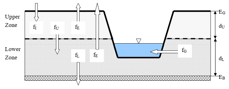
Figure 5-1 Definitional sketch of the two-zone groundwater model.
Flow from the unsaturated upper zone to the saturated lower zone is controlled by a percolation equation for which parameters may either be estimated or calibrated, depending on the availability of the necessary soils data. The upper zone receives vertical inflow from infiltrating rainfall as described in Chapter 4 and can also lose moisture through evapotranspiration. For time steps where the water table has risen to the surface (reducing the unsaturated zone volume to zero), infiltration ceases and runoff is produced by saturation excess.
Losses and outflow from the lower zone consist of deep percolation, saturated zone evapotranspiration, and lateral groundwater flow. The latter is a user-defined power function of water table stage and depth of water in the receiving node of the conveyance system. If the water elevation at the node is higher than the saturated zone water table, back-flow (bank storage) can occur into the saturated zone.
This two-zone representation of surface runoff-groundwater interaction is modeled as follows (refer to Figure 5-1). The ground surface has a known elevation (relative to some fixed reference) of *EG* (ft) and the bottom of the saturated zone has a known elevation of *EB* (ft). The unsaturated upper zone has a varying moisture content denoted as θ. The lower zone is completely saturated, and therefore its moisture content is fixed at the soil porosity φ. Aside from θ, the other principal unknown is *dL*, the depth of the saturated zone (i.e., the water table depth). Because the depth from the ground surface to the bottom of the lower zone is fixed, the depth of the unsaturated zone *dU* is simply \(E_{G} - E_{B} - d_{L}\).
The depths of the two zones and the water content of the upper zone are controlled by the volumetric water fluxes shown in Figure 5-1. These fluxes, expressed as volume per unit horizontal area per unit time (or ft/sec internally in SWMM), consist of the following:
fI = infiltration from the subcatchment surface, which is the value computed in Chapter 4 multiplied by the fraction of pervious area *Fperv*. fEU = evapotranspiration from the upper zone, which is a fixed fraction of the unused surface evaporation, \(e \times F_{perv}\).
fU = percolation from the upper to lower zone, which depends on the upper zone moisture content θ and upper zone depth *dU*.
fEL = evapotranspiration from the lower zone, which is a function of the depth of the upper zone *dU*.
fL = percolation from the lower zone to deep groundwater, which depends on the lower zone depth *dL*.
fG = lateral groundwater seepage to the conveyance network which depends on the lower zone depth *dL* as well as the water surface elevation in the receiving node.
Computation of these fluxes will be discussed subsequently, but keep in mind that they are either supplied externally or depend on the unknown variables θ , *dU* and *dL*.
The conservation of mass equation for the upper zone can be written as:
\[\frac{\partial V_{U}}{\partial t} = f_{UZ}\]
(5-1)
where *VU* is the volume of water per unit area (ft) in the upper zone and fUZ (ft/sec) is the net influx rate to the upper zone. The latter is equal to:
\[f_{UZ} = f_{I} - f_{EU} - f_{U}\]
(5-2)
The conservation of mass equation for the lower zone is:
\[\frac{\partial V_{L}}{\partial t} = f_{LZ}\]
(5-3)
where *VL* is the volume of water per unit area (ft) in the lower zone and fLZ is the net influx rate into the lower zone given by:
\[f_{LZ} = f_{U} - f_{EL} - f_{L} - f_{G}\]
(5-4)
A third equation is needed to express the change in lower zone depth as a function of change in lower zone volume:
\[(\phi - \theta)\frac{\partial d_{L}}{\partial t} = \frac{\partial V_{L}}{\partial t}\]
(5-5)
This equation accounts for the fact that as the lower zone contracts or expands it is consuming or vacating a portion of upper zone which has a moisture content of θ. For example, if the lower zone expands it absorbs an amount of moisture θ contained in the upper zone. Because the lower zone always has a fixed moisture content of φ, its expansion must be accompanied by a volume increase of φ - θ to make up the difference. Substituting Equation 5-5 into 5-3 results in the following expression for the rate of change of the lower zone depth:
\[\frac{\partial d_{L}}{\partial t} = \frac{f_{LZ}}{(\phi - \theta)}\]
(5-6)
And since \(V_{U} = \theta d_{U}\), Equation 5-1 can be expanded as:
\[\frac{\partial V_{U}}{\partial t} = \frac{\partial\left( \theta d_{U} \right)}{\partial t} = d_{U}\frac{\partial\theta}{\partial t} + \theta\frac{\partial d_{U}}{\partial t} = f_{UZ}\]
(5-7)
From the relation \(d_{U} = E_{G} - E_{B} - d_{L}\) and Equation 5-6 one can write:
\[\frac{\partial d_{U}}{\partial t} = - \frac{\partial d_{L}}{\partial t} = - \frac{f_{LZ}}{(\phi - \theta)}\]
(5-8)
Substituting this into 5-7 and solving for [Figure image not available in this format] gives:
\[\frac{\partial\theta}{\partial t} = \frac{\theta f_{LZ} + (\phi - \theta)f_{UZ}}{(\phi - \theta)\left( E_{G} - E_{B} - d_{L} \right)}\]
(5-9)
Equations 5-6 and 5-9 form a system of ordinary differential equations in θ and *dL* that can be solved using a standard fifth-order Runge-Kutta integration routine with adaptive step size control (Press et al., 1992). The integration is applied over each runoff time step as the calculation of surface runoff unfolds (see Section 3.4). The initial conditions at time zero are *dL = dL0* and *θ = θ0* where *dL0* is the initial depth of the saturated zone and *θ0* is the initial moisture content of the unsaturated zone. Additional conditions that must be honored during each time step Δt are:
This simple two-zone groundwater model has a number of limitations that the reader should be aware of:
In order to integrate the groundwater conservation of mass equations over a succession of time steps one must compute the various flux terms that transport water into and out of the two sub-surface zones. This section discusses how each of these terms is modeled.
The surface infiltration flux rate fI is set equal to the runoff infiltration rate f computed as described in Chapter 4, multiplied by the fraction of the subcatchment that is pervious, *Fperv*. (The groundwater zones extend over the entire subcatchment area while surface infiltration is computed only for the pervious portion of this area.) fI is considered a constant quantity over the current runoff time step Δt. However, it is not allowed to exceed a rate that would fill up the available pore volume of the upper unsaturated zone by the end of the time step. This rate fImax can be computed as:
\[f_{Imax} = \frac{d_{U}(\phi - \theta)}{\Delta t} + f_{U}\]
(5-10)
where fU is an estimate of the percolation flux rate between the upper and lower zones at the start of the time period and is computed using the equations given in Section 5.3.2 below. Thus if the infiltration computed from the surface runoff calculation, fI, is greater than fImax then fI is set equal to fImax and the infiltration rate used for surface runoff calculations is reduced to fI/Fperv.
Evapotranspiration (ET) from the upper zone, fEU, represents soil moisture lost via cover vegetation and by direct evaporation from the pervious area of the subcatchment. This ET is a portion of the overall potential evaporation rate for the study area supplied externally to the program using the data sources described in Section 2.5. The order in which this overall rate is allocated to the various types of ET losses is as follows: 1) land surface evaporation, 2) upper zone evapotranspiration, and 3) lower zone transpiration. Upper zone ET is computed as:
\(f_{EU} = min(e_{\max} - e_{s},\ UEF \times e_{\max})\) (5-11)
where UEF is a fraction of available evaporation that is apportioned to the upper zone, \(e_{\max} = eF_{perv}\), e is the maximum potential evaporation rate (ft/s) available for the current time period supplied externally, *Fperv* is the fraction of the subcatchment that is pervious, and *es* is the evaporation loss (ft/s) seen by any rainfall and ponded water on the pervious subcatchment surface. The latter is computed as:
\[e_{s} = \frac{\min(e, d_a/\Delta t)}{F_{perv}}\]
(5-12)
where *da* is the depth of available moisture on the pervious area of the subcatchment (ft). The latter quantity was evaluated at Step 3b of the procedure used to compute surface runoff (see Section 3.4). In addition, fEU is set to 0 whenever the upper zone soil moisture drops below the wilting point or when the infiltration rate fI > 0 (since it is assumed that the resulting vapor pressure will be high enough to prevent any evapotranspiration from the unsaturated zone). Note the need to adjust the surface evaporation rates by *Fperv* because although evaporation from the groundwater zone extends over the entire subsurface area of the subcatchment it can only be released through the pervious portion of the subcatchment.
Lower zone evapotranspiration, fEL, represents the ET, or more properly just the transpiration, lost from the saturated lower zone. It is assumed to vary in direct proportion to the distance that the water table sits above some reference level below which no ET can occur. In equation form:
\[f_{EL} = (1 - UEF)e_{\max}\frac{DEL - d_{U}}{DEL}\]
(5-13)
where DEL is the depth from the ground surface below which no lower zone ET is possible (ft). The fEL value computed from (5-12) is constrained to be non-negative and be no greater than \(e_{\max} - e_{s} - f_{EU}\).
Percolation, fU, represents the flow of water from the unsaturated zone to the saturated zone, and apart from possible bank storage is the only inflow for the saturated zone. The percolation equation is formulated from Darcy's Law for unsaturated flow, in which the hydraulic conductivity, K, is a function of the moisture content, θ. For one-dimensional, vertical flow, Darcy's Law may be written as:
\[v = K(\theta)\frac{dh}{dz}\]
(5-14)
where:
v = velocity (specific discharge), positive in the downward direction of z (ft/s), z = vertical coordinate with respect to the ground surface (ft),
K(θ) = hydraulic conductivity (ft/s),
θ = moisture content (dimensionless), and
h = hydraulic potential or head (ft).
The hydraulic potential is the sum of the elevation (gravity) and pressure heads,
\[h = z + \psi\]
(5-15)
where ψ = soil water tension (negative pressure head) in the unsaturated zone. Note that the wetting front suction, *ψS, used in the Green-Ampt equations is simply the average value of *ψ along the wetting front during the infiltration process. Equating vertical velocity to percolation, and differentiating the hydraulic potential, h, yields:
\[f_{U} = K(\theta)(1 + \frac{d\psi}{dz})\]
(5-16)
A choice is customarily made between using the tension, ψ, or the moisture content, θ, as parameters in equations for unsaturated zone water flow. Since the quantity of water in the unsaturated zone is identified by θ in previous equations, it is the choice here. Parameter ψ can be related to θ if the characteristics of the unsaturated soil are known. Thus, for use in Equation 5-16, the derivative is:
\[\frac{d\psi}{dz} = \frac{d\psi}{d\theta}\frac{d\theta}{dz}\]
(5-17)
However, since θ is assumed constant throughout the upper zone, \(\frac{d\theta}{dz = 0}\) and the percolation flux becomes simply:
\[f_{U} = K(\theta)\]
(5-18)
The hydraulic conductivity K as a function of moisture content θ is approximated functionally in the moisture range of interest as:
\[K(\theta) = K_{s}e^{- (\phi - \theta)HCO}\]
(5-19)
where *KS* is the saturated hydraulic conductivity (ft/s) and HCO is a calibration parameter. Estimates of HCO can be made from soil test data and some examples will be given in section 5.4 below. Substituting 5-19 into 5-16 yields the final form of the percolation rate expression:
\[f_{U} = K_{s}e^{- (\phi - \theta)HCO}\]
(5-20)
If the moisture content θ is less than or equal to field capacity θFC, then the percolation rate becomes zero. This limit is in accordance with the concept of field capacity as the drainable soil water that cannot be removed by gravity alone (Hillel, 1982, p. 243). Once θ drops below field capacity, it can only be further reduced by upper zone evapotranspiration (to a lower bound of the wilting point moisture content).
Deep percolation, fL, represents a lumped sink term for un-quantified losses from the saturated zone. The two primary losses are assumed to be percolation through the confining layer and lateral outflow to somewhere other than the conveyance system. The arbitrarily chosen equation for deep percolation is:
\[f_{L} = DP\frac{d_{L}}{E_{G} - E_{B}}\]
(5-21)
where DP is a recession coefficient derived from inter-event water table recession curves. The dependence of fL on *dL* allows it to be a function of the static pressure head above the confining layer.
Groundwater discharge, fG, (lateral flow per horizontal area of the groundwater region or cfs/ft²) represents lateral flow from the saturated zone to elements in the conveyance system. The latter can take the form of an adjacent stream or channel or under-drains in the groundwater region, with the recognition that groundwater discharge in SWMM is actually to (and from) nodes, not directly to channels or pipes. (If need be, refer back to Section 1.2 for a description of how SWMM represents a conveyance system as a network of links and nodes.) If a channel receives groundwater, then its upstream node is used instead. The flux equation for groundwater discharge takes on the following general form:
\[f_{G} = A1\left( d_{L} - h^* \right)^{B1} - A2\left( h_{SW} - h^* \right)^{B2} + A3d_{L}h_{SW}\]
(5-22)
where:
fG = groundwater flow rate (cfs/ft²), hSW = height of surface water above the bottom of the groundwater zone (ft),
h* = reference height above the bottom of the groundwater zone (ft),
A1, B1 = groundwater flow coefficient and exponent,
A2, B2 = surface water flow coefficient and exponent,
A3 = surface-groundwater interaction coefficient.
Figure 5-2 illustrates the meaning of each of the water depths used in this expression. The reference height h^ is typically chosen as the height to the bottom of the conveyance system node, but other choices are possible. The coefficients A1, A2, and A3 are units-dependent. As shown here A1 has units of ft(1-*B1*)/s, A2 has units of ft(1-*B2*)/s, while A3 is in (ft-s)-1. In an actual SWMM input data set the user would use coefficients that produce flow rates measured in cfs/ac for US units or cms/ha for metric units. SWMM automatically converts these input coefficients so that Equation 5-22 is evaluated internally using cfs/ft².
The particular function form of Equation 5-22 was selected in order to approximate various horizontal flow conditions as will be illustrated later. The reference height h* sets the minimum elevation at which groundwater flow is possible (i.e., fG becomes 0 when either *dL* or hSW is below h*). If h* is not explicitly set by the user it defaults to the height of the receiving node's invert as shown in Figure 5-2. Also note that the conveyance system node receiving groundwater flow need not be the same node that receives runoff from the subcatchment that lies above the groundwater zones.
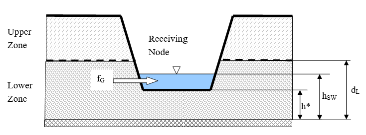
Figure 5-2 Heights used to compute lateral groundwater flow rate.
The effects of channel water on groundwater flow can be dealt with in two different ways. The first option entails setting hSW (water surface height in the receiving node) to a constant value greater than or equal to h* and A2, B2 and/or A3 to values greater than zero. If this method is chosen, then the user is specifying an average tailwater influence over the entire run to be used at each time step.
The second option uses the actual water surface height at the receiving node, as determined during the flow routing calculations for the conveyance system (flow routing is discussed in Volume II of this manual). In this case hSW can vary over time and the value used in Equation 5-22 is the flow routing result at the start of the current time step.
Note that when conditions warrant, the groundwater flux, fG, can be negative, simulating flow into the aquifer from the channel, in the manner of bank storage. An exception occurs when A3 ≠ 0, since the surface water – groundwater interaction term is usually derived from groundwater flow models that assume unidirectional flow (examples are provided below). Otherwise, to ensure that negative fG values will not occur, one can make A1 greater than or equal to A2, B1 greater than or equal to B2, and A3 equal to zero. More examples of adjusting the flow coefficients and exponents to reproduce specific physical conditions are provided in section 5.5 on Parameter Estimation.
SWMM also has the ability to employ custom user-defined equations for the lateral groundwater discharge flux (fG) and the deep percolation flux (fL). These can be any well-formed mathematical expression relating fG (in cfs/acre or cms/ha) or fL (in in/hr or mm/hr) to any of several pre-defined variables. More details can be found in the SWMM 5 User's Manual (US EPA, 2010).
For example, a two-stage linear reservoir model for lateral groundwater outflow could be expressed as:
**fG = 0.001*Hgw + 0.05*(Hgw-5)*STEP(Hgw-5)**
where Hgw is the pre-defined variable name used for height of the groundwater table (i.e., *dL* as used here) and STEP is a special cutoff function pre-defined as STEP(x) = 0 if x < 0 and is 1 otherwise. The expression says that there is some small background flow out of the aquifer that is proportional to the height of the saturated zone plus a second larger source of outflow that only occurs when the saturated zone height exceeds 5. It would not be possible to express this type of behavior using just the standard discharge equation 5-21.
An example for deep percolation flux might be
**fL = 2.5*Hgw - 0.1**
which is equivalent to expressing fL through Darcy's Law as:
\(f_{L} = K_{c}(d_{L} - H_{c})/d_{c}\)
where *Kc* is the hydraulic conductivity of the confining layer beneath the shallow aquifer, *dc* is the thickness of this layer, and *Hc* is the hydraulic head below the layer. The values 2.5 and 0.1 in the user-defined expression would come from knowing specific values of *Kc*, *dc*, and *Hc*.
Groundwater computations are a sub-procedure implemented as part of SWMM's runoff calculations. They are made at each runoff time step, for each subcatchment that has a groundwater component, immediately after infiltration over the subcatchment's pervious area has been computed. This is at Step 3c of the runoff procedure described in Section 3.4. The detailed steps involved are described in the sidebar below.
Computational Scheme for Groundwater
The following variables are assumed known at the start of each time step of length Δt (sec) for each subcatchment with a defined groundwater component:
Available from surface runoff calculations:
Available from conveyance system flow routing calculations:
Groundwater state variables:
In addition, the following constants are also assumed known for each subcatchment:
Soil properties:
Elevations:
Groundwater flow constants:
Note that at time 0 the state variables θ and dL are initialized with user-supplied values.
With the above information in hand, the following steps are used to update each subcatchment's groundwater system:
\[f_{Umax} = \frac{d_U(\phi - \theta_{FC})}{\Delta t}\]
where dU = EG – EB – dL.\[e_s = \min[e, d_a/\Delta t] F_{perv}\]
\[f_{Imax} = \frac{d_U(\phi - \theta)}{\Delta t} - f_U\]
and set fI to the smaller of f×Fperv (as computed by the infiltration routine) and fImax. If fI = fImax then reduce f to fI/Fperv for use in the runoff routine after it returns from the groundwater calculations.\[f_{Gmax} = \frac{d_L \phi}{\Delta t}\]
(cannot release more than what is stored)\[f_{Gmin1} = -\frac{d_U(\phi - \theta)}{\Delta t}\]
(cannot accept more than can be stored)\[f_{Gmin2} = \frac{(V_N/\Delta t)}{A}\]
(cannot accept more than node can release)\[f_{Gmin} = \max[f_{Gmin1}, f_{Gmin2}]\]
(the maximum is used because fGmin is negative) where A is the total area of the subcatchment.\[\frac{\partial\theta}{\partial t} = \frac{\theta f_{LZ} + \phi f_{UZ}}{\phi(E_G - E_B - d_L)}\]
\[\frac{\partial d_L}{\partial t} = \frac{f_{LZ}}{\phi}\]
where fUZ = fI - fEU - fU and fLZ = fU - fEL - fL - fG. The solution updates the values of θ and dL at time t to new values at time t + Δt. The RK5 routine requires that the right-hand sides of these equations be evaluated at intermediate values of θ and dL. The equations used to evaluate the flux terms that comprise fUZ and fLZ are summarized below:| Term | Equation | Constraints |
|---|---|---|
| fI | Step 4 above | |
| fEU | 5-11 | 0 when θ ≤ θWP or fI > 0 |
| fEL | 5-13 | between 0 and emax - es - fEU |
| fU | 5-20 | 0 when θ ≤ θFC; otherwise between 0 and fUmax |
| fL | 5-21 or user-supplied | between 0 and DP (for Eq. 5-21) |
| fG | 5-22 or user-supplied | between fGmin and fGmax |
Estimates of the following constants are required in order to implement the two-zone groundwater model:
SWMM uses an Aquifer object to bundle together a common set of soil moisture limits, ET coefficients, and percolation parameters that can be shared by any number of subcatchments. This helps to reduce the amount of input values that must be supplied to the program. Multiple Aquifer objects can be defined to accommodate variations in subsurface conditions across the study area. On the other hand, a distinct set of groundwater discharge constants must be supplied for each subcatchment that experiences groundwater flow.
Porosity (φ) is defined as the volumetric water content of a soil (volume of water per total volume) when its pore spaces are at saturation. No distinction is made here between the actual porosity and the apparent porosity, which includes trapped air, since no mechanism exists for adjusting for the latter and the difference is usually minor (5-10 %). Porosity is a critical parameter because of its role in determining moisture storage. Field capacity (*θFC*) is usually considered to be the amount of water a well-drained soil holds after free water has drained off, or the maximum amount it can hold against gravity (Linsley et al., 1982; SCS, 1991). This occurs at soil moisture tensions of from 0.1 to 0.7 atmospheres, depending on soil texture. Moisture content at a tension of 1/3 atmosphere is often used. The wilting point (or permanent wilting point) (*θWP*), is the soil moisture content at which plants can no longer obtain enough moisture to meet transpiration requirements; they wilt and die unless water is added to the soil. The moisture content at a tension of 15 atmospheres is accepted as a good estimate of the wilting point (Linsley et al., 1982; Jensen et al., 1990; SCS, 1991). The field capacity must be greater than the wilting point and less than the porosity. The general relationship among soil moisture parameters is shown in Figure 5-3.
Figure 5-3 Relation between soil moisture limits and soil texture class (Schroeder et al., 1994).
Data for soil moisture limits are available from the NRCS, agricultural extension offices and university soil science departments. Generalized values for porosity, field capacity, and wilting point are available from several published sources. Tables 5-1 and 5-2 contain representative values of field capacity and wilting point from Linsley et al. (1982) and the U.S. Army Corps of Engineers (1956), respectively. Table 5-3 is a summary of average parameter values for different soil types presented by Rawls et al. (1983). These data were published primarily to provide estimates of the Green-Ampt infiltration parameters that were listed previously in Table 4-7, but also included values for field capacity and wilting point.
Table 5-1 Volumetric moisture content at field capacity and wilting point (derived from Linsley et al., 1982)
| Soil Type | Field Capacity (ft³/ft³) | Wilting Point (ft³/ft³) |
|---|---|---|
| Sand | 0.08 | 0.03 |
| Sandy loam | 0.17 | 0.07 |
| Loam | 0.26 | 0.14 |
| Silt loam | 0.28 | 0.17 |
| Clay loam | 0.31 | 0.19 |
| Clay | 0.36 | 0.26 |
| Peat | 0.56 | 0.30 |
*Fraction moisture content = fraction dry weight × dry density / density of water.
Table 5-2 Volumetric moisture content at field capacity and wilting point (U.S. Army Corps of Engineers, 1956)
| Soil Type | Field Capacity (ft³/ft³) | Wilting Point (ft³/ft³) |
|---|---|---|
| Sand | 0.10 | 0.03 |
| Fine sand | 0.12 | 0.03 |
| Sandy loam | 0.16 | 0.05 |
| Fine sandy loam | 0.22 | 0.07 |
| Silty loam | 0.28 | 0.12 |
| Light clay loam | 0.30 | 0.13 |
| Clay loam | 0.32 | 0.15 |
| Heavy clay loam | 0.33 | 0.18 |
| Clay | 0.33 | 0.21 |
Table 5-3 Average moisture limits and saturated hydraulic conductivity for different soil types (Rawls et al., 1983)
| Soil Type | Porosity (ft³/ft³) | Field Capacity (ft³/ft³) | Wilting Point (ft³/ft³) | Saturated Hydraulic Conductivity (in/hr) |
|---|---|---|---|---|
| Sand | 0.437 | 0.062 | 0.024 | 4.74 |
| Loamy sand | 0.437 | 0.105 | 0.047 | 1.18 |
| Sandy loam | 0.453 | 0.190 | 0.085 | 0.43 |
| Loam | 0.463 | 0.232 | 0.116 | 0.13 |
| Silt loam | 0.501 | 0.284 | 0.135 | 0.26 |
| Sandy clay loam | 0.398 | 0.244 | 0.136 | 0.06 |
| Clay loam | 0.464 | 0.310 | 0.187 | 0.04 |
| Silty clay loam | 0.471 | 0.342 | 0.210 | 0.04 |
| Sandy clay | 0.430 | 0.321 | 0.221 | 0.02 |
| Silty clay | 0.479 | 0.371 | 0.251 | 0.02 |
| Clay | 0.475 | 0.378 | 0.265 | 0.01 |
Schroeder et al. (1994) developed more extensive tables of soil moisture limits that were used to provide default parameter values for the U.S. EPA HELP (Hydrological Evaluation of Landfill Performance) model. They were derived from the large data base of soil measurements reported by Rawls et al. (1982). Table 5-4 contains a version of the HELP table for uncompacted, low-density soils while Table 5-5 does the same for compacted, moderate-density soils. The soils in these tables are referred to by both their USDA and Unified Soil Classification System (USCS) textures. Table 5-6 explains the abbreviations used for these classifications.
Table 5-4 Default properties of low-density soils used in the EPA HELP model (from Rawls et al. (1982) as reported in Schroeder et al. (1994))
| Soil Texture Class | USDA | USCS | Porosity (ft³/ft³) | Field Capacity (ft³/ft³) | Wilting Point (ft³/ft³) | Saturated Hydraulic Conductivity (in/hr) |
|---|---|---|---|---|---|---|
| CoS | CoS | SP | 0.417 | 0.045 | 0.018 | 14.173 |
| S | S | SW | 0.437 | 0.062 | 0.024 | 8.220 |
| FS | FS | SW | 0.457 | 0.083 | 0.033 | 4.394 |
| LS | LS | SM | 0.437 | 0.105 | 0.047 | 2.409 |
| LFS | LFS | SM | 0.457 | 0.131 | 0.058 | 1.417 |
| SL | SL | SM | 0.453 | 0.190 | 0.085 | 1.020 |
| FSL | FSL | SM | 0.473 | 0.222 | 0.104 | 0.737 |
| L | L | ML | 0.463 | 0.232 | 0.116 | 0.524 |
| SiL | SiL | ML | 0.501 | 0.284 | 0.135 | 0.269 |
| SCL | SCL | SC | 0.398 | 0.244 | 0.136 | 0.170 |
| CL | CL | CL | 0.464 | 0.310 | 0.187 | 0.091 |
| SiCL | SiCL | CL | 0.471 | 0.342 | 0.210 | 0.060 |
| SC | SC | SC | 0.430 | 0.321 | 0.221 | 0.047 |
| SiC | SiC | CH | 0.479 | 0.371 | 0.251 | 0.035 |
| C | C | CH | 0.475 | 0.378 | 0.251 | 0.035 |
Table 5-5 Default properties of moderate-density soils used in the EPA HELP model (Schroeder et al. (1994))
| Soil Texture Class | USDA | USCS | Porosity (ft³/ft³) | Field Capacity (ft³/ft³) | Wilting Point (ft³/ft³) | Saturated Hydraulic Conductivity (in/hr) |
|---|---|---|---|---|---|---|
| L | L | ML | 0.419 | 0.307 | 0.180 | 0.027 |
| SiL | SiL | ML | 0.461 | 0.360 | 0.203 | 0.013 |
| SCL | SCL | SC | 0.365 | 0.305 | 0.202 | 0.004 |
| CL | CL | CL | 0.437 | 0.373 | 0.266 | 0.005 |
| SiCL | SiCL | CL | 0.445 | 0.393 | 0.277 | 0.003 |
| SC | SC | SC | 0.400 | 0.366 | 0.288 | 0.001 |
| SiC | SiC | CH | 0.452 | 0.411 | 0.311 | 0.002 |
| C | C | CH | 0.451 | 0.419 | 0.332 | 0.001 |
Table 5-6 Soil texture abbreviations
| USDA Soil Texture | Unified Soil Classification System | ||
|---|---|---|---|
| Symbol | Meaning | Symbol | Meaning |
| S | Sand | S | Sand |
| Si | Silt | M | Silt |
| C | Clay | C | Clay |
| L | Loam (mixture of sand, silt, clay and humus) | P | Poorly graded |
| Co | Coarse | W | Well graded |
| F | Fine | H | High plasticity or compressibility |
| L | Low plasticity or compressibility |
More specific soil parameter estimates can be obtained from the NRCS Soil Survey reports available for each county in the U.S. These were discussed previously in Section 4.1. An excerpt from the Physical Properties portion of one such report was displayed in Figure 4-1. Using the bulk density *ρb* value provided in these reports, an estimate of the porosity can be derived from:
\[\phi = 1 - \frac{\rho_{b}}{\rho_{s}}\]
(5-23)
where:
*φ*Â = porosity, *ρb* = bulk density (mass of dried soil to total volume of soil and voids), g/cm³,
*ρs* = soil particle density, typically in range 2.6-2.7 g/cm³ for quartz particles.
As an example, the bulk density for the Woodburn silt loam listed in Figure 4-1 is 1.35 g/cm³ and using a *ρs* = 2.65 g/cm³ in Equation 5-23 yields a φ* = 0.49.* This corresponds well with the general value of 0.501 for silt loam given in Tables 5-4 and 5-5. Carrying the example further, when Primary Characterization Data are obtained for Woodburn silt loam (Benton County, Oregon) from the NRCS web site, the moisture content at 1500 kPa (15 atm) for the surface layer is 13.7 percent, a good estimate for the wilting point for this soil (Jensen et al., 1990). Similarly, the moisture content listed at 33 kPa (0.33 atm) representing the field capacity is about 28 percent.
Another approach to estimating soil moisture limits are the empirical equations developed by Saxton and Rawls (2006) from a data base of over 2,000 soil samples. These utilize the standard soil grain size classification of percent sand, silt, and clay along with organic content to estimate a soil's porosity, field capacity and wilting point. Sand and clay percentages should be determined using a grain size distribution chart and particle sizes defined by the U.S. Department of Agriculture textural soil classification system. According to this system, sand particles range in size from 0.05 mm to 2.0 mm, silt particles from 0.002 mm to 0.05 mm, and clay particles are less than 0.002 mm. The relevant equations are listed in Table 5-7.
The SPAW computer model (http://hydrolab.arsusda.gov/SPAW), used to analyze the hydrology of agricultural fields, contains a stand-alone calculator that implements these equations within a graphical user interface and also makes adjustments for salinity, gravel content and degree of compaction (see Figure 5-4). Table 5-8 shows the results from this calculator for the same soil classes listed previously in Table 5-3. For the Woodburn silt loam discussed earlier, the program yields moisture limits of 13.7, 32.1 and 48.2 percent for the wilting point, field capacity, and porosity, respectively.
Table 5-7 Regression equations for soil moisture limits (Saxton and Rawls, 2006)
| Soil Moisture Limit¹ | Equation² |
|---|---|
| **Wilting Point (θWP)** | θWP = θ1500t + (0.14θ1500t - 0.02) where θ1500t = -0.024S + 0.487C + 0.006OM + 0.005(S × OM) - 0.013(C × OM) + 0.068(S × C) + 0.031 |
| **Field Capacity (θFC)** | θFC = θ33t + (1.283θ33t² - 0.374θ33t - 0.015) where θ33t = -0.251S + 0.195C + 0.011OM + 0.006(S × OM) - 0.027(C × OM) + 0.452(S × C) + 0.299 |
| Porosity (φ) | φ = θFC + θ(S-33) - 0.097S + 0.043 where θ(S-33) = θ(S-33)t + 0.636θ(S-33)t - 0.107 and θ(S-33)t = 0.278S + 0.034C + 0.022OM - 0.018(S × OM) - 0.027(C × OM) - 0.584(S × C) + 0.078 |
¹Moisture limits are fractional volumes.
²S = weight fraction of sand, C = weight fraction of clay, OM = percent organic matter.
Figure 5-4 SPAW\'s soil water characteristics calculator.
Table 5-8 Regression estimates of soil moisture limits from the SPAW calculator
| Soil Type | Porosity (ft³/ft³) | Field Capacity (ft³/ft³) | Wilting Point (ft³/ft³) | Saturated Hydraulic Conductivity (in/hr) |
|---|---|---|---|---|
| Sand | 0.463 | 0.094 | 0.050 | 4.49 |
| Loamy sand | 0.457 | 0.121 | 0.057 | 3.59 |
| Sandy loam | 0.450 | 0.179 | 0.081 | 1.98 |
| Loam | 0.458 | 0.267 | 0.126 | 0.73 |
| Silt loam | 0.482 | 0.321 | 0.137 | 0.48 |
| Sandy clay loam | 0.432 | 0.283 | 0.183 | 0.31 |
| Clay loam | 0.472 | 0.350 | 0.213 | 0.18 |
| Silty clay loam | 0.510 | 0.379 | 0.210 | 0.23 |
| Sandy clay | 0.440 | 0.371 | 0.260 | 0.03 |
| Silty clay | 0.532 | 0.416 | 0.278 | 0.15 |
| Clay | 0.488 | 0.420 | 0.299 | 0.03 |
*For 2.5% organic matter content by weight.
The two parameters that govern the percolation rate between the upper and lower groundwater zones are the soil's saturated hydraulic conductivity *KS* and the coefficient HCO that characterizes the exponential decrease in hydraulic conductivity with decreasing moisture content. The most accurate way of estimating these parameters is from laboratory tests that measure hydraulic conductivity K as a function of soil moisture content θ for the particular soil under consideration. Such data for three particular soils – sand, sandy loam, and silty loam – are shown in Figure 5-5. They were generated from disturbed soil samples under desaturation (draining) conditions (see Brooks and Corey (1964) and Laliberte et al. (1966)). In some cases (e.g., sand), K(θ) may range through several orders of magnitude. Soils data of this type are becoming more readily available; for example, soil science departments at universities often publish such information (e.g., Carlisle et al., 1981).
Figure 5-5 Measured hydraulic conductivity for three soils.
When soil data like this are available, *KS* and HCO can be estimated by fitting Equation 5-20 to the data, i.e., fitting a straight line to the plot of the logarithm of K versus θ. The fits are not optimal over the entire data range because the fit is only performed for the high moisture content region between field capacity and porosity.
When laboratory data are not available general estimates of *KS* based on soil texture class can be obtained from Tables 5-3, 5-4, and 5-5. Another alternative is the regression equation derived by Saxton and Rawls (2006) from the same soils data base used to derive the moisture limit equations listed in Table 5-7. The equation for *KS* (in/hr) is:
\[K_{s} = 76{(\phi - \theta_{FC})}^{(3 - \lambda)}\]
(5-24)
where \(\lambda = 0.262ln\left( \frac{\theta_{FC}}{\theta_{WP}} \right)\) and φ = soil porosity, *θFC* = field capacity and *θWP* = the wilting point. This equation is also included in the SPAW soil water characteristics calculator described in the previous section and shown in Figure 5-4. The estimates of *KS* it produces for the different soil classes are shown in Table 5-8. For the Woodburn silt loam soil in Section 5.5.1, it estimates a saturated hydraulic conductivity of 0.48 in/hr (see Figure 5-4). This value falls within the range of 0.2 - 2.0 in/hr (1.4 - 14 µm/sec) listed in the Physical Properties report of Figure 4-1.
HCO can be estimated by utilizing Campbell's theoretical power law relation (Campbell, 1974) as described in Saxton and Rawls (2006):
\[K(\theta) = K_{S}\left( \frac{\theta}{\phi} \right)^{3 + 2/\lambda}\]
(5-25)
One can then estimate a value for HCO that gives a best fit between Equation 5-19 and Equation 5-25 as θ ranges between φ and *θFC. Figure 5-6 shows one such fit for the soil limits associated with the Woodburn Silt Loam discussed earlier (*φ = 0.482, *θFC* = 0.321, and *θWP* = 0.137). The data points come from evaluating Equation 5-25 for a series of different moisture levels θ. The line of best fit that passes through the origin has a slope of 28.864 which would be the estimate of HCO for this soil.
Figure 5-6 Fitting SWMM's hydraulic conductivity equation to a power law equation.
Repeating this fitting process for the sand and clay content of the various standard soil classes under a variety of organic contents, using the SPAW calculator to estimate the associated moisture limits, produced the following regression estimate for HCO:
\(HCO = 0.48(\% Sand) + 0.85(\% Clay)\) R² = 0.99 (5-26)
The resulting HCO values for the different soil classes are shown in Table 5-9.
A third percolation parameter, DP, governs the rate of at which water is lost from the lower saturated zone by seepage through a confining layer into a deeper groundwater aquifer. DP essentially represents the saturated hydraulic conductivity of this confining bottom layer and will therefore typically have very low values, similar to those for compacted clay soils. If water table measurements are available, DP can also be estimated from the rate at which the water table elevation drops over a prolonged dry period.
Table 5-9 Estimated HCO for different soil types
| Soil Type | Percent Sand | Percent Clay | HCO |
|---|---|---|---|
| Sand | 92 | 5 | 48 |
| Loamy sand | 82 | 6 | 44 |
| Sandy loam | 65 | 10 | 40 |
| Loam | 42 | 18 | 35 |
| Silt loam | 20 | 20 | 27 |
| Sandy clay loam | 60 | 28 | 53 |
| Clay loam | 33 | 34 | 45 |
| Silty clay loam | 10 | 34 | 34 |
| Sandy clay | 52 | 42 | 61 |
| Silty clay | 7 | 47 | 43 |
| Clay | 30 | 50 | 57 |
The two evapotranspiration parameters used by the groundwater routine are CET, the fraction of the available evaporation apportioned to the upper unsaturated zone, and DET, the depth from the ground surface below which no lower zone ET is possible (ft). The total rate available for subsurface evaporation is the external evaporation rate supplied to the program for the current month or day (see Section 2.5) minus the rate used for surface evaporation (Equation 5-12). The CET parameter determines what fraction of this remaining evaporation rate is used in the upper subsurface zone. In general, higher CET values will be associated with looser soils, lower water table elevations, and surface vegetation with shallow root zones.
The amount of ET available to the saturated lower zone is 1 – CET of the total subsurface available ET. The fraction of this amount actually utilized is proportional to the height that the water table rises above a depth DET measured from the ground surface. DET is the maximum depth from which water may be removed by evapotranspiration. Because the lower zone is saturated, ET losses reflect mainly plant transpiration. Where surface vegetation is present, DET should at least equal the expected average depth of root penetration. The influence of plant roots usually extends somewhat below the depth of root penetration because of capillary suction to the roots. The depth of capillary draw to the surface without vegetation may be 4 to 8 inches for sands, about 8 to 18 inches in silts, and in clays about 12 to 60 inches. Rooting depth is dependent on many factors -- species, moisture availability, maturation, soil type, and plant density. In humid areas where moisture is readily available near the surface, grasses may have rooting depths of 6 to 24 inches. In drier areas, the rooting depth is very sensitive to plant species and to the depth to which moisture is stored and may range from 6 to 48 inches. The evaporative zone depth would be somewhat greater than the rooting depth. The local Agricultural Extension Service office can provide information on characteristic rooting depths for vegetation in specific areas. Table 5-10 presents values of DET for different combinations of soil type and ground cover that were derived from unsaturated-saturated flow simulations (Shah et al., 2007).
Table 5-10 DET (in feet) for different soil types and land cover (Shah et al., 2007)
| Soil Type | Bare Soil | Grass | Forest |
|---|---|---|---|
| Sand | 2 | 5 | 8 |
| Loamy Sand | 2 | 6 | 9 |
| Sandy Loam | 4 | 8 | 11 |
| Sandy clay loam | 7 | 10 | 13 |
| Sandy clay | 7 | 10 | 13 |
| Loam | 9 | 12 | 15 |
| Silty clay | 11 | 14 | 17 |
| Clay loam | 13 | 17 | 20 |
| Silt loam | 14 | 17 | 20 |
| Silt | 14 | 17 | 21 |
| Silty clay loam | 15 | 18 | 21 |
| Clay loam | 20 | 23 | 27 |
The groundwater discharge constants A1, B1, A2, B2, and A3 appear in Equation 5-22 and determine the rate of groundwater exchange with a specific node in the conveyance system. The equation is repeated here for easy reference:
\[f_{G} = A1\left( d_{L} - h^* \right)^{B1} - A2\left( h_{SW} - h^* \right)^{B2} + A3d_{L}h_{SW}\]
(5-27)
where the heights *dL*, *hSW, and h are defined in Figure 5-2. Because of its general nature this equation can assume a variety of functional forms. Several specific examples will now be discussed.
[Linear Reservoir]{.underline}
The saturated groundwater zone can be thought of as a storage reservoir whose lateral outflow is linearly proportional to the water table depth *dL*. Two cases are possible – with and without surface water interaction. Without surface water interaction, the groundwater flow rate is simply:
\[f_{G} = A1\left( d_{L} - h^* \right)\]
(5-28)
In terms of Equation 5-27 this implies that A1 > 0, B1 = 1, and A2 = A3 = 0. Note that the user-supplied value of A1 would be expressed as cfs/ac-ft for US units and cms/ha-m for metric units. With surface water interaction, the groundwater flow rate is proportional to the difference between the groundwater table height and the surface water height:
\[f_{G} = A1\left( d_{L} - h_{SW} \right)\]
(5-29)
which can be achieved with A1 = A2 > 0, B1 = B2 = 1, and A3 = 0. A1 would have the same units as before (cfs/ac-ft or cms/ha-m). Because both of these cases are empirical simplifications, A1 would have to be determined through model calibration against observed groundwater table and conveyance system head measurements.
[Dupuit-Forcheimer Lateral Seepage]{.underline}
Under the assumption of uniform infiltration and horizontal flow by the Dupuit-Forcheimer approximation, the relationship between water table elevation and groundwater flow rate for the configuration shown in Figure 5-7 is (Bouwer, 1978, p.51):
\[f_{G} = \frac{K_{S}}{2L^{2}}\left( h_{1}^{2} - h_{2}^{2} \right)\]
(5-30)
where *KS* is the saturated hydraulic conductivity and the other parameters are defined in Figure 5-7.
While *h2* is the same as the surface water height *hSW*, *h1* is the [maximum]{.underline} groundwater table height. The height *dL* that SWMM computes is only an average over the catchment. One can, however, assume this average is equivalent to the average of *h1* and *h2*, i.e.:
\[d_{L} = \frac{h_{1} + h_{2}}{2}\]
(5-31)
so that \(h_{1} = 2d_{L} - h_{2}\). Substituting this and \(h_{2} = h_{SW}\) into Equation 5-30 and simplifying terms results in:
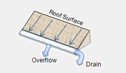
Figure 5-7 Definition sketch for Dupuit-Forcheimer seepage to an adjacent channel.
\[f_{G} = \left( \frac{2K_{S}}{L^{2}} \right)d_{L}^{2} - \left( \frac{2K_{S}}{L^{2}} \right)d_{L}h_{SW}\]
(5-32)
Comparing Equation 5-32 with Equation 5-27 shows that the two will be equivalent if A1 = -A3 *= 2KS / L², A2 = 0,* B1 = 2, and h* =
[Hooghoudt's Equation for Tile Drainage]{.underline}
The geometry of a tile drainage installation is illustrated in Figure 5-8. Hooghoudt's relationship (Bouwer, 1978, p. 295) among the indicated parameters is
\[f_{G} = \left( 2D_{e} + m \right)4K_{S}\frac{m}{L^{2}}\]
(5-33)
where *De* = effective depth of the impermeable layer below the drain center, and the other parameters are defined in Figure 5-8. *De* is less than or equal to *b0* in Figure 5-8 and is a function of *b0, drain diameter, and drain spacing *L; the complicated relationship is given by Bear (1972, p. 412) and graphed by Bouwer (1978, p. 296).
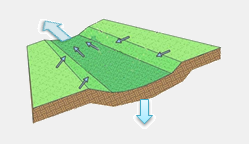
Figure 5-8 Definition sketch for Hooghoudt's method for flow to circular drains.
From Figure 5-8, the maximum rise of the water table, m, is:
\[m = h_{1} - b_{0}\]
(5-34)
Once again approximating the average water table depth above the impermeable layer by:
\[d_{L} = \frac{h_{1} + b_{0}}{2}\]
(5-35)
results in:
\[m = 2\left( d_{L} - b_{0} \right)\]
(5-36)
Substituting 5-36 into 5-33 gives:
\[f_{G} = \left( \frac{16K_{S}}{L^{2}} \right)\left\lbrack \left( d_{L} - b_{0} \right)^{2} - D_{e}b_{0} + D_{e}d_{L} \right\rbrack\]
(5-37)
This can be written in a format compatible with the general groundwater discharge equation 5-27 as follows:
\[f_{G} = A1{(d_{L} - h^*)}^{2} - A2 + A3d_{L}h_{SW}\]
(5-38)
where
\(A1 = 16K_{S}/L^{2}\),
\(B1 = 2\),
\(A2 = A1D_{e}b_{0}\),
\(B2 = 0\),
\(A3 = A1(\frac{D_{e}}{b_{0}})\),
h* is set equal to *b0* and a constant value of *hSW* only slightly higher than *b0* is used.
The internal units of both A1 and A3 are (ft-s)^-1^ while A2 has units of ft/s. In terms of the program input though, where fG is expressed as flow per acre (or per hectare), the units on A1 and A3 would be would be ft/s/ac (or m/s/ha) and for A2 would be ft³/s/ac (or m³/s/ha). Since A3 ≠ 0, flow back into the groundwater zone would not be allowed should *dL* drop below *b0*. The mathematics of drainage to ditches or circular drains is complex; several alternative formulations are described by van Schilfgaarde (1974).
A simple numerical example will help illustrate the effect that groundwater can have on the runoff generated from a subcatchment. It is a variation of the runoff example used in Section 3.10 which consists of a single relatively flat, completely pervious subcatchment containing a well-drained Group B soil that is subjected to a 2-inch, 6-hour rain event. The subsurface zone beneath the subcatchment extends to a depth of 6 feet and its initial water table height is 3.5 feet. Because a conveyance node is required to complete a groundwater model, a single such node is included that receives both the surface runoff and the groundwater flow from the subcatchment. Its invert elevation is 0.5 feet above the initial water table level. The Linear Reservoir form of the groundwater discharge equation without surface water interaction is used. Table 5-11 summarizes the pertinent parameters for this example. The initial moisture content of the unsaturated zone is 0.4, midway between fully saturated and fully drained.
Table 5-11 Parameters used in groundwater example
| Item | Parameter | Value |
|---|---|---|
| Subcatchment | Percent Impervious | 0 |
| Percent Slope | 0.5 | |
| Width (ft) | 140 | |
| Roughness | 0.1 | |
| Depression Storage (in) | 0.05 | |
| Rainfall Event | Duration (hr) | 6.0 |
| Total Depth (in) | 2.0 | |
| Time-to-Peak / Duration | 0.375 | |
| Evaporation Rate (in/hr) | 0.0 | |
| Horton Infiltration | Initial Capacity (in/hr) | 1.2 |
| Ultimate Capacity (in/hr) | 0.1 | |
| Decay Coefficient (hr⁻¹) | 2.0 | |
| Groundwater | Porosity | 0.5 |
| Field Capacity | 0.3 | |
| Wilting Point | 0.15 | |
| Saturated Hydraulic Conductivity (in/hr) | 0.1 | |
| Conductivity Curve Parameter (HCO) | 12.0 | |
| Deep Percolation Constant (DP) | 0.002 | |
| Reference Depth (h*) (ft) | 4.0 | |
| GW Flow Coefficient (A1) (cfs/ac-ft) | 0.5 | |
| GW Flow Exponent (B1) | 1.0 | |
| A2, A3 and B2 | 0.0 |
The surface runoff and the groundwater flow seen by the outlet node over a 24-hour simulation period are shown in Figure 5-9. The surface runoff is unaffected by inclusion of the subsurface zones, since the upper zone never fully saturates. Its hydrograph looks the same as for the example in Section 3.10 (see the pervious curve in Figure 3-12). However, as the infiltrated water percolates through the upper soil zone, the depth of the lower saturated zone rises and begins to produce groundwater outflow into the receiving node. This outflow continues long after the surface runoff ceases, creating an extended recession limb on the total outflow hydrograph.
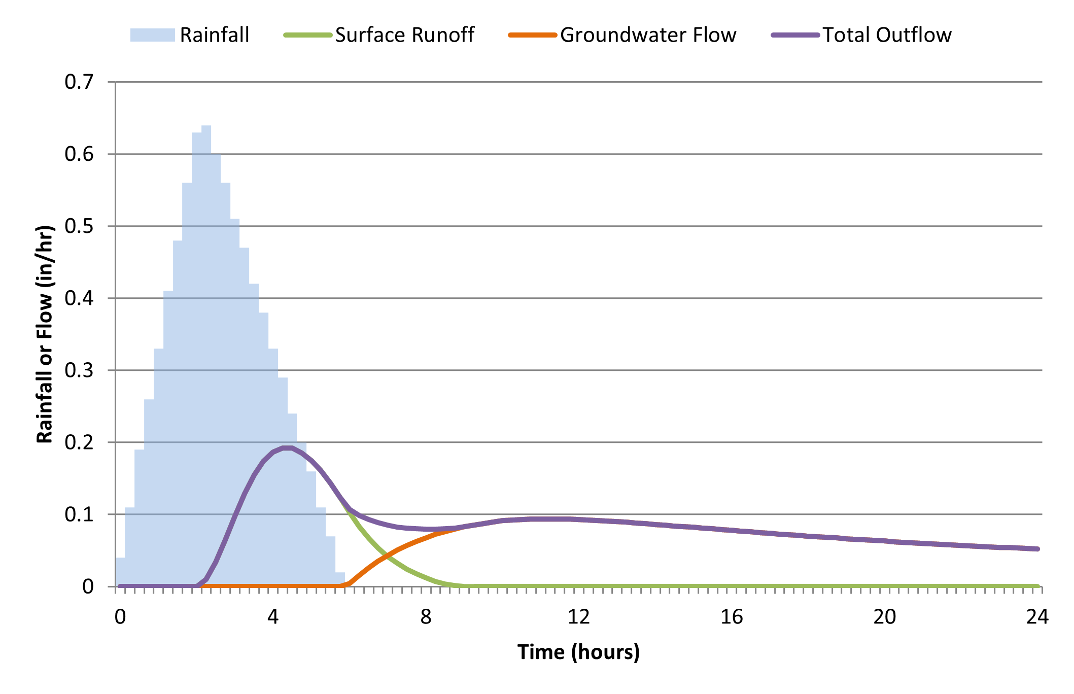
Figure 5-9 Surface runoff and groundwater flow for the illustrative groundwater example.
 1.13.2