 |
OpenSWMM Engine
6.0.0-alpha.4
Data-oriented, plugin-extensible SWMM Engine (6.0.0-alpha.4)
|
|
OpenSWMM Engine
6.0.0-alpha.4
Data-oriented, plugin-extensible SWMM Engine (6.0.0-alpha.4)
|
Infiltration is the process by which rainfall penetrates the ground surface and fills the pores of the underlying soil (Akan and Houghtalen, 2003). It often accounts for the largest portion of rainfall losses over pervious areas. Theoretically, infiltration is governed by the Richards equation (Richards, 1931) which requires that the relationship between soil permeability and pore water tension as a function of soil moisture content be known. The difficulty in solving this highly nonlinear partial differential equation makes it unsuitable for use in a general purpose model like SWMM, especially for long-term continuous simulations. Engineers have developed several simpler algebraic infiltration models that capture the general dependence of infiltration capacity on soil characteristics and the volume of previously infiltrated water during the course of a storm event. Because there is no universal agreement as to which model is best, SWMM allows the user to choose from among four of the most widely used methods: Horton's method, a modified Horton method, the Green-Ampt method, and the Curve Number method.
No matter which infiltration method is used, the parameters that define the method are highly dependent on the type and condition of the soil being infiltrated. The NRCS (Natural Resources Conservation Service, formerly the Soil Conservation Service or SCS) has classified most soils into Hydrologic Soil Groups, A, B, C, and D, depending on their limiting infiltration capacities. Well drained, sandy soils are "A"; poorly drained, clayey soils are "D," as described in Table 4-1. Every soil in the United States has an A-D classification, or sometimes a dual classification, such as B/D, meaning drained (artificially) and undrained (natural) condition.
The group assigned to specific types of soils and locations can be found by consulting:
Additional soil characterization (physics and chemical) data are available at the aforementioned web sites.
**Table 4-1 Hydrologic soil group meanings (NRCS, 2009, Chapter 7)**
| Group | Meaning |
|---|---|
| A | Low runoff potential. Soils having high infiltration rates even when thoroughly wetted and consisting chiefly of deep, well to excessively drained sands or gravels. |
| B | Soils having moderate infiltration rates when thoroughly wetted and consisting chiefly of moderately deep to deep, moderately well to well-drained soils with moderately fine to moderately coarse textures. E.g., shallow loess, sandy loam. |
| C | Soils having slow infiltration rates when thoroughly wetted and consisting chiefly of soils with a layer that impedes downward movement of water, or soils with moderately fine to fine textures. E.g., clay loams, shallow sandy loam. |
| D | High runoff potential. Soils having very slow infiltration rates when thoroughly wetted and consisting chiefly of clay soils with a high swelling potential, soils with a permanent high water table, soils with a clay-pan or clay layer at or near the surface, and shallow soils over nearly impervious material. |
The best source of information about a particular soil type is the Soil Survey Interpretation, available from a local NRCS office in the U.S. Data for soils in each county are often summarized in a county soil survey document; the latter is often available in a local Soil and Water Conservation District. Because printed versions of these documents are increasingly difficult to obtain, on-line access is more likely (http://soils.usda.gov/survey/). Of particular interest is the "Physical Properties" report that includes parameters of interest regarding infiltration. This report may be downloaded for any soil, as illustrated in Figure 4-1. These data include saturated hydraulic conductivity, for instance. Other potentially useful reports include:
In short, the NRCS provides an invaluable resource for information on soils and drainage of soils. The agency's data are ever more valuable as they increasingly reside on-line on the Web.
Figure 4-1 Physical properties for Woodburn silt loam, Benton County, Oregon.
Horton's method is empirical in nature and is perhaps the best known of the infiltration equations. Many hydrologists have a "feel" for the best values of its three parameters despite the fact that little published information is available. In its usual form it is applicable only to events for which the rainfall intensity always exceeds the infiltration capacity; however, the modified form used in SWMM is intended to overcome this limitation. The Horton method has been a part of SWMM since the program was first released (Metcalf and Eddy et al., 1971a).
Horton (1933, 1940) proposed the following exponential equation to predict the reduction in infiltration capacity over time as observed from field measurements:
\[f_{p} = f_{\infty} + \left( f_{0} - f_{\infty} \right)e^{- k_{d}t}\]
(4-1)
where:
fp = infiltration capacity into soil (ft/sec)
f∞ = minimum or equilibrium value of fp (at t = ∞) (ft/sec)
f0 = maximum or initial value of fp (at t = 0) (ft/sec)
t = time from beginning of storm (sec)
kd = decay coefficient (sec-1).
Equation 4-1 is sketched in Figure 4-2 and can be derived theoretically from the Richards equation under the proper set of assumptions (Eagleson, 1970). Note that actual infiltration will be the lesser of actual rainfall and infiltration capacity:
\[f(t) = min\left\lbrack f_{p}(t),\ i(t) \right\rbrack\]
(4-2)
where:
f = actual infiltration into the soil (ft/sec) i = rainfall intensity (ft/sec).
: Thus for the case illustrated in Figure 4-2 runoff would be intermittent.
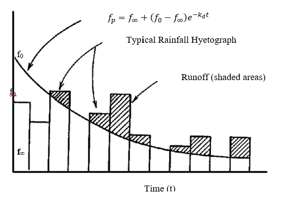
Figure 4-2 The Horton infiltration curve
Typical values for parameters fo and f∞ are usually greater than typical rainfall intensities. Thus, when Equation 4-1 is used such that fp is a function of time only, the exponential term will cause fp to decrease even if rainfall intensities are very light, as sketched in Figure 4-2. This results in a reduction in infiltration capacity regardless of the actual amount of entry of water into the soil.
To correct this problem, the integrated form of Horton's equation 4-1 is used in SWMM:
\[F\left( t_{p} \right) = \int_{0}^{t_{p}}{f_{p}dt = f_{\infty}t_{p} + \frac{\left( f_{0} - f_{\infty} \right)}{k_{d}}\left( 1 - e^{- k_{d}t_{p}} \right)}\]
(4-3)
where F is the cumulative infiltration capacity at time tp in feet. This function is plotted in Figure 4-3 where it is assumed that actual infiltration has been equal to fp over all time t. As noted before, there will in fact be times when infiltration f is less than fp, so that the true cumulative infiltration will be:
\[F(t) = \int_{0}^{t}{\min\left\lbrack f_{p},\ i \right\rbrack d\tau}\]
(4-4)
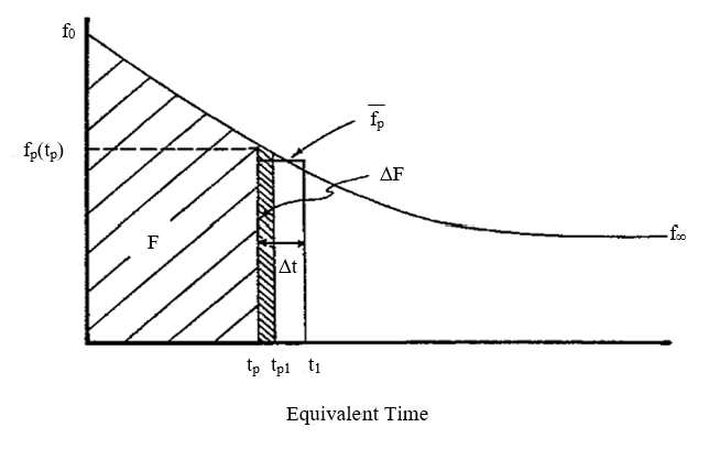
Figure 4-3 Cumulative infiltration F as the area under the Horton curve
Equations 4-3 and 4-4 can thus be used to define the time tp along the Horton curve at which the next value of fp can be found. That is, F is updated with the actual infiltration f over the current time step and then the following equation, with tp as the only unknown, is solved:
\[F = f_{\infty}t_{p} + \frac{\left( f_{0} - f_{\infty} \right)}{k_{d}}\left( 1 - e^{- k_{d}t_{p}} \right)\]
(4-5)
Once the new tp is known, the infiltration capacity fp for the next time step can be found from Equation 4-1.
An additional optional parameter Fmax can be specified that limits the total volume of water that can infiltrate the soil. When cumulative infiltration exceeds this value, saturation conditions exist, and no more infiltration occurs; the land surface behaves as if it were impermeable. Thus F(t) in Equation 4-4 is not allowed to exceed Fmax.
For simulations that consist of multiple storm events over a set period of time, infiltration capacity will be regenerated (recovered) during dry weather periods. With Horton's method, SWMM performs this function whenever a subcatchment is dry – meaning it receives no precipitation and has no ponded surface water – according to the hypothetical drying curve sketched in Figure 4-4:
\[f_{p} = f_{0} - \left( f_{0} - f_{\infty} \right)e^{- k_{r}\left( t - t_{w} \right)}\]
(4-6)
where:
kr = decay coefficient for the recovery curve (sec-1) tw = hypothetical projected time at which fp = f∞ on the recovery curve (sec).
New values of tp are then generated as indicated in Figure 4-4 as recovery proceeds. For example, let tpr be the tp value at which recovery begins with fr as the corresponding infiltration capacity. According to the recovery curve,
\[f_{r} = f_{0} - \left( f_{0} - f_{\infty} \right)e^{- k_{r}\left( t_{pr} - t_{w} \right)}\]
(4-7)
one can compute tw as:
\[t_{w} = t_{pr} - \frac{1}{k_{r}}\ln\left( \frac{f_{0} - f_{\infty}}{f_{0} - f_{r}} \right)\]
(4-8)
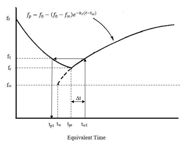
Figure 4-4 Regeneration (recovery) of infiltration capacity during dry time steps
Then after a recovery time to tw1 = tpr + Δ*t*, the new infiltration capacity f1 is found from:
\[f_{1} = f_{0} - \left( f_{0} - f_{\infty} \right)e^{- k_{r}\left( t_{w1} - t_{w} \right)}\]
(4-9)
Finally, the new equivalent time tp1 on the infiltration curve from which the infiltration process would re-start under a wet condition is:
\[t_{p1} = \frac{1}{k_{d}}\ln\left( \frac{f_{0} - f_{\infty}}{f_{1} - f_{\infty}} \right)\]
(4-10)
These steps can be combined into the following equation:
\[t_{p1} = \frac{1}{k_{d}}\ln\left\lbrack 1 - e^{- k_{r}\mathrm{\Delta}t}\left( 1 - e^{- k_{d}t_{pr}} \right) \right\rbrack\]
(4-11)
On succeeding time steps, tp1 may be substituted for tpr, and tp2 substituted for tp1, etc. Note that fp has reached its maximum value of f0 when tp = 0.
Although this recovery method gives sensible results, it is somewhat unsatisfactory inasmuch as there is no dependence of infiltration recovery on evapotranspiration (ET). Drying of the soil through ET and deep infiltration should influence the recovery of infiltration capacity, but these mechanisms are replaced in SWMM by the more empirical approach just discussed.
The detailed computational scheme for computing Horton infiltration for each subcatchment within a study area over a single time step of a simulation is presented in the sidebar below.
The parameters that a user must supply for each subcatchment for the Horton infiltration method are:
f0 - the maximum or initial infiltration capacity (in/hr or mm/hr),
f∞ - the minimum or equilibrium infiltration capacity (in/hr or mm/hr),
kd - the decay coefficient (hr-1),
kr - the regeneration coefficient (days-1), and, optionally,
Fmax - the maximum infiltration volume (in or mm).
Conversions between the user-supplied units of these parameters (such as in, mm or hr) and those used internally (ft and sec) are handled automatically by the program.
Although the Horton equation is probably the best-known of the several infiltration equations available, there is little to help the user select values of parameters f0 and kd for a particular application. (Fortunately, some guidance can be found for the value of f∞.). Since the actual values of f0 and kd (and often f∞.) depend on the soil, vegetation, and initial moisture content, ideally these parameters should be estimated using results from field infiltrometer tests for a number of sites of the watershed and for a number of antecedent wetness conditions. An example of Horton parameters for Georgia soils is given in Table 4-2 (Rawls et al., 1976). Horton's (1940) estimates are shown in Table 4-3. Skaggs and Khaleel (1982) provide Horton-type decay curves on the basis of theoretical estimates.
Table 4-2 Horton parameters for selected Georgia soils (Rawls et al., 1976)
| Soil Type | f∞ (in/hr) | f₀ (in/hr) | kd (hr⁻¹) |
|---|---|---|---|
| Alpha loamy sand | 1.40 | 19.0 | 38.29 |
| Carnegie sandy loam | 1.77 | 14.77 | 19.64 |
| Cowarts loamy sand | 1.95 | 15.28 | 10.65 |
| Dothan loamy sand | 2.63 | 3.47 | 1.40 |
| Fuquay pebbly loamy sand | 2.42 | 6.24 | 4.70 |
| Leefield loamy sand | 1.73 | 11.34 | 7.70 |
| Robersdale loamy sand | 1.18 | 12.41 | 21.75 |
| Stilson loamy sand | 1.55 | 8.11 | 6.55 |
| Tooup sand | 1.80 | 23.01 | 32.71 |
Table 4-3 Horton parameters provided by Horton (1940)
| Soil and Cover | f∞ (in/hr) | f₀ (in/hr) | kd (hr⁻¹) |
|---|---|---|---|
| Standard agricultural (bare) | 0.24 – 8.9 | 11.4 | 96 |
| Standard agricultural (turfed) | 8.2 – 11.8 | 36.7 | 48 |
| Peat | 0.82 – 11.8 | 13.3 | 108 |
| Fine sandy clay (bare) | 0.82 – 1.0 | 8.6 | 120 |
| Fine sandy clay (turfed) | 4.1 – 1.2 | 27.4 | 84 |
If it is not possible to use field data to find estimates of f0, f∞, and kd for each subcatchment, the following guidelines should be helpful. Often, NRCS data may be used directly. For instance, for the two upper horizons (soil layers) of Woodburn silt loam (Figure 4-1), saturated hydraulic conductivity is listed as 4 - 14 micrometers per second, or 0.6 - 2.0 in/hr (14 - 50 mm/hr). Unfortunately, this wide range in values is commonly encountered among soil survey data. Fortunately, the range also serves as a reminder that infiltration rates are notoriously variable in space as well as in time and should not be considered "exact." Note that saturated hydraulic conductivity is the more appropriate word for parameter KS, also termed "permeability" on older soil survey interpretation tables.
**Minimum Infiltration Capacity (f∞)**
The Horton parameter f∞ is essentially equal to saturated hydraulic conductivity, KS, that is, f∞ ≈ KS. The f∞ value is also the limiting infiltration rate when water is ponded on the surface, at low depths. Generalized estimates for KS will also be discussed in conjunction with the Green-Ampt infiltration method later in this chapter and are the best source of values for f∞ in the absence of site-specific data.
Alternatively, values for f∞ according to Musgrave (1955) are given in Table 4-4. To help select a value within the range given for each soil group, the user should consider the texture of the layer of least hydraulic conductivity in the profile. Depending on whether that layer is sand, loam, or clay, the f∞ value should be chosen near the top, middle, and bottom of the range respectively. For example, the data sheet for Woodburn silt loam identifies it as being in Hydrologic Soil Group B, which puts the estimate of f∞ into the range of 0.15 - 0.30 in/hr (3.8 -7.6 mm/hr), much lower than the KS value discussed above. Examination of the texture of the layers in the soil profile indicates that they are silty in nature, suggesting that the estimate of the f∞ value should be in the low end of the range, say 0.15 - 0.20 in/hr (3.8 - 5.1 mm/hr). A sensitivity test on the f∞ value will indicate the importance of this parameter to the overall result; in fact, f∞ is usually the most sensitive of the three Horton curve parameters.
Table 4-4 Values of f∞ for Hydrologic Soil Groups (Musgrave, 1955)
| Hydrologic Soil Group | f∞ (in/hr) |
|---|---|
| A | 0.45 - 0.30 |
| B | 0.30 - 0.15 |
| C | 0.15 - 0.05 |
| D | 0.05 - 0 |
Caution should be used in applying values from Table 4-4 to sandy soils (group A) since reported KS values are often much higher. For instance, sandy soils in Florida can have KS values from 7 to 18 in/hr (180 - 450 mm/hr) (Carlisle et al., 1981). Unless the water table rises to the surface, minimum infiltration capacity will be very high, and rainfall rates will almost always be less than f∞, leading to little or no overland flow from such soils.
**Decay Coefficient (kd)**
For any field infiltration test the rate of decrease (or "decay") of infiltration capacity from the initial value depends on the initial moisture content. Thus the kd-value determined for the same soil will vary from test to test. It is postulated here that, if f0 is always specified in relation to a particular soil moisture condition (e.g., dry), and for moisture contents other than this the time scale is changed accordingly (i.e., time "zero" is adjusted to correspond with the constant f0), then kd can be considered a constant for the soil independent of initial moisture content. Put another way, this means that infiltration curves for the same soil, but different antecedent conditions, can be made coincident if they are moved along the time axis. Butler (1957) makes a similar assumption.
Values of kd found in the literature (Overton and Meadows, 1976; Wanielista, 1978; Maidment, 1993; ASCE, 1996) range from 0.67 to 120 hr-1. Nevertheless most of the values cited appear to be in the range 3 - 6 hr-1. The evidence is not clear as to whether there is any relationship between soil texture and the kd value although several published curves seem to indicate a lower value for sandy soils. If no field data are available, an estimate of 4 hr-1 could be used. Use of such an estimate implies that, under ponded conditions, the infiltration capacity will fall 98 percent of the way towards its minimum value in the first hour, a not uncommon observation. Rates of decay of infiltration for several values of kd are shown in Table 4-5.
Table 4-5 Rate of decay of infiltration capacity for different values of kd
| kd (hr⁻¹) | Percent of decline of infiltration capacity towards limiting value f∞ after 1 hour |
|---|---|
| 2 | 76 |
| 3 | 95 |
| 4 | 98 |
| 5 | 99 |
**Initial Infiltration Capacity (f0)**
The initial infiltration capacity, f0 depends primarily on soil type, initial moisture content, and surface vegetation conditions. For example, Linsley et al. (1982) present data that show, for a sandy loam soil, a 60 to 70 percent reduction in the f0 value due to wet initial conditions. They also show that lower f0 values apply for a loam soil than for a sandy loam soil. As to the effect of vegetation, Jens and McPherson (1964, pp. 20.20-20.38) list data that show that dense grass vegetation nearly doubles the infiltration capacities over those measured for bare soil surfaces.
For the assumption to hold that the decay coefficient kd is independent of initial moisture content, f0 must be specified for the dry soil condition. For long-term continuous simulations SWMM automatically adjusts the effective f0 value as part of the infiltration capacity regeneration routine. However, for a single-event simulation, the user must specify the f0 value for the storm in question, which may be less than the value for dry soil conditions.
Published values of f0 vary depending on the soil, moisture, and vegetation conditions for the particular test measurement. The f0 values listed in Table 4-6 can be used as a rough guide. Interpolation between the values may be required.
Table 4-6 Representative values for f₀
A. DRY soils (with little or no vegetation):
B. DRY soils (with dense vegetation):
C. MOIST soils (change from dry f₀ value required for single event simulation only):
**Regeneration Coefficient (kr)**
For continuous simulation, infiltration capacity will be regenerated (recovered) during dry weather according to Equation 4-6. Instead of asking the user to supply a value for kr, SWMM instead asks for an estimate of drying time Tdry in days. This is the time it takes for a saturated soil to fully recover to a dry state. Drying times are typically longer than wetting times, implying k~r~ < k~d~. On well-drained porous soils (e.g., medium to coarse sands), recovery of infiltration capacity is quite rapid and could well be complete in a couple of days. For heavier soils, the recovery rate is likely to be slower, say 7 to 14 days. The choice of the value can also be related to the interval between a heavy storm and wilting of vegetation.
The Green-Ampt method (discussed below in Section 4.4), bases its recovery time solely on the soil's saturated hydraulic conductivity KS. Adopting its approach produces the following estimate for Tdry in days:
\[T_{dry} = \frac{3.125}{\sqrt{K_{s}}}\]
(4-12)
where KS is expressed in in/hr. Thus this equation predicts a drying time of 2 days for a sandy soil with KS = 2.0 in/hr versus 10 days for a clay soil with KS of 0.1 in/hr.
Since mathematically, the exponential term in Equation 4-6 would require an infinite amount of time to allow infiltration capacity to return to its initial value f0, SWMM considers "full recovery" to occur when 98 percent of the difference between the initial and minimum capacities has been achieved. Thus from Equation 4-6 (for kr in days-1),
\[0.02\left( f_{0} - f_{\infty} \right) = \left( f_{0} - f_{\infty} \right)e^{- k_{r}T_{dry}}\]
(4-13)
which leads to the following estimate of kr expressed in days-1:
\[k_{r} = \frac{- ln(0.02)}{T_{dry}} = \frac{3.912}{T_{dry}}\]
(4-14)
This computation of kr from a user-supplied value of Tdry and its subsequent conversion from days-1 to sec-1 is done internally by SWMM.
A. O. Akan developed a modified version of the Horton infiltration method (Akan, 1992; Akan and Houghtalen, 2003) that has been added as a separate infiltration option in SWMM 5. The method uses the same parameters as the original Horton method but instead of tracking the time along the Horton decay curve it uses the cumulative infiltration volume in excess of the minimum infiltration rate as its state variable. It assumes that part of the infiltrating water will percolate deeper into the soil at the minimum infiltration rate (commonly taken as the soil's saturated hydraulic conductivity). As a result, it is the difference between the actual and minimum infiltration rates that accumulates just below the surface that causes infiltration capacity to decrease with time. This method is purported to give more accurate infiltration estimates when low rainfall intensities occur.
The modified method starts with the same exponential decay equation as the original Horton method:
\[f_{p} = f_{\infty} + \left( f_{0} - f_{\infty} \right)e^{- k_{d}t}\]
(4-15)
where all symbols have been previously defined.
As with the original Horton method, the actual infiltration rate f is the smaller of fp and the rainfall rate i. Integrating Equation 4-15 from 0 to time t produces the following equation for the cumulative infiltration through time t:
\[F = f_{\infty}t + \frac{\left( f_{0} - f_{\infty} \right)}{k_{d}}\left( 1 - e^{- k_{d}t} \right)\]
(4-16)
Solving for \(e^{- k_{d}t}\) from (4-15) and substituting into (4-16) gives:
\[F = f_{\infty}t + \frac{f_{0} - f_{p}}{k_{d}}\]
(4-17)
and solving for fp gives:
\[f_{p} = f_{0} - k_{d}(F - f_{\infty}t)\]
(4-18)
The last term in parenthesis is equivalent to \(\int_{0}^{t}{\left( f - f_{\infty} \right)dt}\). So one can approximate Eq. (4-18) by
\[f_{p} = f_{0} - {k_{d}F}_{e}\]
(4-19)
where \(F_{e} = \sum_{i}^{}{(f_{i} - f_{\infty})\mathrm{\Delta}t_{i}}\) and \(f_{i}\) is the actual infiltration over a previous time interval \(\mathrm{\Delta}t_{i}\).
Regarding recovery of infiltration capacity during dry periods, one can assume that the instantaneous recovery rate is proportional to the difference between the current capacity and the maximum capacity:
\[\frac{df_{r}}{dt} = k_{r}(f_{0} - f_{r})\]
(4-20)
where \(f_{r}\) represents the infiltration capacity during recovery and \(k_{r}\) is the same regeneration coefficient (1/sec) used in the conventional Horton method. Integrating this equation starting at some time where the infiltration capacity is \(f_{r0}\) produces the following result for the capacity after a recovery time of t:
\[f_{r} = f_{0} - (f_{0} - f_{r0})e^{- k_{r}t}\]
(4-21)
From Eq. 4-19, the cumulative excess infiltration volume corresponding to this capacity, \(F_{er}\), would be:
\[F_{er} = (f_{0} - f_{r})/k_{d}\]
(4-22)
and substituting 4-21 for \(f_{r}\) gives:
\[F_{er} = \frac{\left( f_{0} - f_{r0} \right)}{k_{d}}e^{- k_{r}t}\]
(4-23)
But again from 4-19,
\[(f_{0} - f_{r0})/k_{d} = F_{e}\]
(4-24)
so the new cumulative volume after recovery is simply:
\[F_{er} = F_{e}e^{- k_{r}t}\]
(4-25)
The detailed computational scheme for computing the Modified Horton infiltration rate for each subcatchment within a study area over a single time step of a simulation is presented in the sidebar titled Computational Scheme for Modified Horton Infiltration.
Because the modified Horton method utilizes the same parameters as the original Horton method, the description in section 4.2.4 of how to estimate their values also applies to the modified method.
The Green-Ampt equation (Green and Ampt, 1911) has received considerable attention in recent years. The original equation was for infiltration with excess water at the surface at all times. Mein and Larson (1973) showed how it could be adapted to a steady rainfall input and proposed a way in which the capillary suction parameter could be determined. Chu (1978) has shown the applicability of the equation to the unsteady rainfall situation, using data for a field catchment. The Green-Ampt method was added into SWMM III in 1981 by R.G. Mein and W. Huber (Huber et al., 1981).
The Green-Ampt conceptualization of the infiltration process is one in which infiltrated water moves vertically downward in a saturated layer, beginning at the surface (Figure 4-5). In the wetted zone the moisture content θ is at saturation θs while the moisture content in the un-wetted zone is at some known initial level θi.
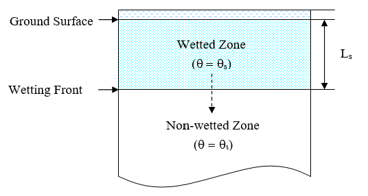
Figure 4-5 Two-zone representation of the Green-Ampt infiltration model (after Nicklow et al., 2006)
The water velocity within the wetted zone is given by Darcy's Law as a function of the saturated hydraulic conductivity KS, the capillary suction head along the wetting front ψS, the depth of ponded water at the surface d, and the depth of the saturated layer below the surface Ls:
\[f_{p} = K_{s}\left\lbrack \frac{d + L_{s} + \psi_{s}}{L_{s}} \right\rbrack\]
(4-26)
The depth of the saturated layer Ls can be expressed in terms of the cumulative infiltration, F, and the initial moisture deficit to be filled below the wetting front, θd = θs - θi as [Figure image not available in this format]. Substituting this into Equation 4-26 and assuming that d is small compared to the other depths gives the Green-Ampt equation for saturated conditions:
\[f_{p} = K_{s}\left\lbrack 1 + \frac{\psi_{s}\theta_{d}}{F} \right\rbrack\]
(4-27)
Equation 4-27 applies only after a saturated layer develops at the ground surface. Prior to this point in time the infiltration capacity will equal the rainfall intensity:
\[f_{p} = i\]
(4-28)
As time increases, one can test whether saturation has been reached by solving 4-27 for F (which will be denoted as Fs) with fp set equal to i and check if this value equals or exceeds the actual cumulative infiltration F:
\[F_{s} = \frac{K_{s}\psi_{s}\theta_{d}}{i - K_{s}}\]
(4-29)
Note that there is no calculation of Fs when i <= K~s~, although F still gets updated during such periods. Finally, in this scheme the actual infiltration f is the same as the potential value fp:
\[f = f_{p}\]
(4-30)
The two equations are illustrated in Figure 4-6 for the situation KS = 0.25 in/hr, ψS = 6.5 in, and θd = 0.20. The initial, flat portion of the curve corresponds to f = i, up to the point where F = F~s~ (Equation 4-29). The remainder of the curve corresponds to the potential rate computed with Equation 4-27. Note that the infiltration rate approaches KS (0.25 in/hr) asymptotically.
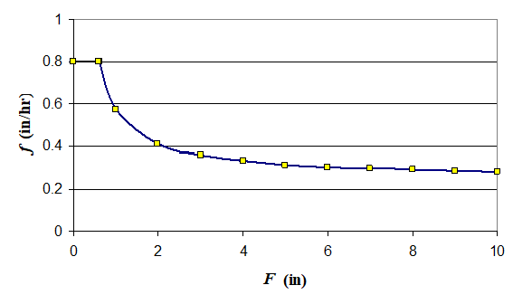
Figure 4-6 Illustration of infiltration capacity as function of cumulative infiltration for the Green-Ampt method
Equation 4-27 shows that the infiltration capacity after surface saturation depends on the infiltrated volume, which in turn depends on the infiltration rates in previous time steps. To avoid numerical errors over long time steps, the integrated form of the Green-Ampt equation is more suitable. That is, fp is replaced by dF/dt and integrated to obtain:
\[F = K_{s} + \psi_{s}\theta_{d}\ln\left( 1 + \frac{F}{\psi_{s}\theta_{d}} \right)\]
(4-31)
If F1 is the known cumulative infiltration at the start of the time step and F2 the unknown cumulative infiltration at the end of the time step then one can write:
\[F_{2} = C + \psi_{s}\theta_{d}\ln\left( F_{2} + \psi_{s}\theta_{d} \right)\]
(4-32)
where \(C = K_{s}\Delta t + F_{1} - \psi_{s}\theta_{d}\ln\left( F_{1} + \psi_{s}\theta_{d} \right)\) is a known constant. Equation 4-32 can be solved numerically for F2. The average infiltration capacity fp over the time step can then be computed as \(\left( F_{2} - F_{1} \right)/\Delta t\).
Evaporation, subsurface drainage, and moisture redistribution between rainfall events decrease the soil moisture content in the upper soil zone and increase the infiltration capacity of the soil. The processes involved are complex and depend on many factors. In SWMM a simple empirical routine (Huber et al., 1981) is used as outlined below; commonly used units are given in the equations to make the description easier to understand. Note that this procedure suffers from the same lack of relationship to ET as does the Horton recovery, discussed earlier.
Infiltration is usually dominated by conditions in the uppermost layer of the soil. The thickness of this layer depends on the soil type; for a sandy soil it could be several inches, for heavy clay it would be less. The equation used to determine the thickness of the layer Lu is:
\[L_{u} = 4\sqrt{K_{s}}\]
(4-33)
where Lu has units of inches and KS is expressed in in/hr. Thus for a high KS of 0.5 in/hr (12.7 mm/hr) the thickness computed by Equation 4-33 is 2.83 inches (71.8 mm). For a soil with a low hydraulic conductivity, say KS = 0.1 in/hr (2.5 mm/hr), the computed thickness is 1.26 inches (32.1 mm). This constant thickness is different from the saturated zone thickness Ls shown in Figure 4-5 which grows over time as infiltration proceeds.
In the Green-Ampt model, the initial soil moisture deficit at the start of a rainfall event determines how much infiltration capacity is available during the event itself. Recall that the moisture deficit θd is the difference between the saturated moisture content θs and the initial moisture content θi. During a dry period the moisture deficit in the upper soil zone, θdu, is regenerated, i.e., its value is increased. Thus SWMM keeps continuous track of this quantity. At the start of a simulation, θdu is set equal to the user-supplied initial value of θdmax. During a wet period when infiltration occurs at a rate f over a time step of Δt, θdu is decreased according to:
\[\theta_{du} \leftarrow \theta_{du} - \frac{f\Delta t}{L_{u}}\]
(4-34)
down to a possible limiting value of 0. During a dry period it increases as follows:
\[\theta_{du} \leftarrow \theta_{du} + k_{r}\theta_{dmax}\Delta t\]
(4-35)
up to a maximum possible value of θdmax , where kr is a recovery constant (hr-1).
One can assume that the recovery constant is also dependent on KS, such that tight, clay soils with low KS take longer to recover than do loose, sandy soils with high KS. The following relationship is used for kr:
\[k_{r} = \frac{\sqrt{K_{s}}}{75}\]
(4-36)
where the constant 75 has units of (in-hr)1/2. Note that the time it would take a fully saturated soil to recovery to its maximum capacity is simply:
\[\frac{1}{k_{r}} = \frac{75}{\sqrt{K_{s}}}\ \]
hours (or \(3.125/\sqrt{K_{s}}\) days).
To complete the recovery process it is necessary to define the minimum amount of time that a soil must remain in recovery before any further rainfall would be considered as an independent event. This time Tr (hr) is computed as:
\[T_{r} = \frac{0.06}{k_{r}} = \frac{4.5}{\sqrt{K_{s}}}\]
(4-37)
Thus when a new period of rainfall occurs after a recovery interval of at least Tr hours, the two-stage Green-Ampt infiltration process is re-started with θd = θdu and F = 0. Figure 4-7 summarizes the functional dependence of the three internally computed recovery parameters Lu, kr, and Tr on the saturated hydraulic conductivity KS.
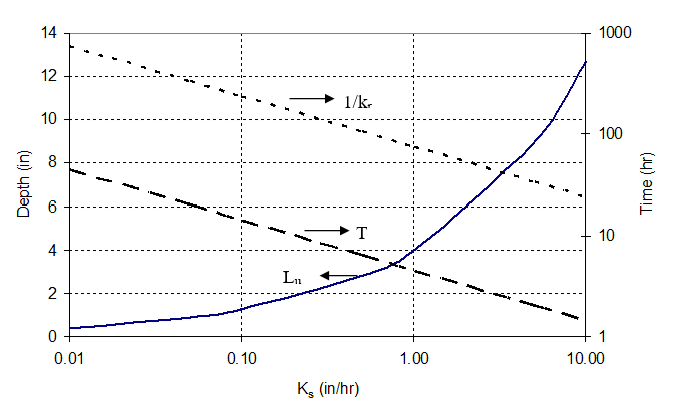
Figure 4-7 Green-Ampt recovery parameters as functions of hydraulic conductivity
The detailed computational scheme for computing the Green-Ampt infiltration rate for each subcatchment within a study area over a single time step of a simulation is presented in the sidebar below.
The soil parameters that a user must supply for each subcatchment for the Green-Ampt infiltration method are:
Conversions between the user-supplied units of these parameters (in (or mm) and hr) and those used internally (ft and sec) are handled automatically by the program.
**Saturated Hydraulic Conductivity (KS)**
Probably the best single source for estimates of saturated hydraulic conductivity (KS) and suction head (ψS) for a wide range of soils – and one that makes use of the Green-Ampt method relatively attractive – is the data by Rawls et al. (1983), shown in Table 4-7. These data were derived from measurements made on roughly 5000 soils across the United States and while they will never be truly site specific, they are certainly consistent and defensible. Although there is considerable variation in the parameter estimates, a good first approximation may be made using the table. Values of hydraulic conductivity may also be used for estimates of the Horton parameter f∞. But the range of values shown for porosity and suction head (the authors do not provide ranges for KS) should be a warning about placing too much faith in such generalized estimates.
The NRCS Soil Survey Physical Data (see Figure 4-1) values for hydraulic conductivity could also be used as a preliminary estimate. A better guide for the KS values is as given for parameter f∞ for the Horton equation; theoretically these parameters (i.e., f∞ and KS) should be equal for the same soil. Note that, in general, the range of KS values encountered will be of the order of tenths of an inch per hour.
Another source of conductivity estimates is the regression equation developed by Saxton and Rawls (2006) that predicts KS from the sand, clay and organic matter content of a soil. See Section 5.5.2 of the Groundwater chapter for more details.
Table 4-7 Green-Ampt parameters for different soil classes (Rawls et al., 1983)
(Numbers in parentheses are ± one standard deviation from the parameter value shown.)
| Soil Class | Porosity, φ | Effective Porosity, φe* | Wetting Front Suction Head, ψs (in) | Saturated Hydraulic Conductivity, Ks (in/hr) |
|---|---|---|---|---|
| Sand | 0.437 (0.374–0.500) | 0.417 (0.354–0.480) | 1.95 (0.38–9.98) | 4.74 |
| Loamy sand | 0.437 (0.363–0.506) | 0.401 (0.329–0.473) | 2.41 (0.53–11.00) | 1.18 |
| Sandy loam | 0.453 (0.351–0.555) | 0.412 (0.283–0.541) | 4.33 (1.05–17.90) | 0.43 |
| Loam | 0.463 (0.375–0.551) | 0.434 (0.334–0.534) | 3.50 (0.52–23.38) | 0.13 |
| Silt loam | 0.501 (0.420–0.582) | 0.486 (0.394–0.578) | 6.57 (1.15–37.56) | 0.26 |
| Sandy clay loam | 0.398 (0.332–0.464) | 0.330 (0.235–0.425) | 8.60 (1.74–42.52) | 0.06 |
| Clay loam | 0.464 (0.409–0.519) | 0.309 (0.279–0.501) | 8.22 (1.89–35.87) | 0.04 |
| Silty clay loam | 0.471 (0.418–0.524) | 0.432 (0.347–0.517) | 10.75 (2.23–51.77) | 0.04 |
| Sandy clay | 0.430 (0.370–0.490) | 0.321 (0.207–0.435) | 9.41 (1.61–55.20) | 0.02 |
| Silty clay | 0.479 (0.425–0.533) | 0.423 (0.334–0.512) | 11.50 (2.41–54.88) | 0.02 |
| Clay | 0.475 (0.427–0.523) | 0.385 (0.269–0.501) | 12.45 (2.52–61.61) | 0.01 |
*Effective porosity is the difference between the porosity φ and the residual moisture content φr that remains after a saturated soil is allowed to drain thoroughly.
Urban soils are usually highly disturbed (Pitt et al., 1999, 2001; Pitt and Voorhees, 2000). Construction has often occurred on or nearby the locations in question, and soils may be compacted from their natural state. Alternatively, soils are sometimes imported for horticultural purposes. Such imported soils (e.g., for lawns) may exhibit relatively high infiltration rates. The parameter estimates discussed previously are based on data for undisturbed soils, e.g., using Natural Resources Conservation Service (NRCS) data. Parameters for natural, undisturbed soils are likely to overestimate the infiltration characteristics for urban soils. Modelers should bear in mind that only site-specific infiltrometer and/or soil physics tests can determine local infiltration properties, and that high spatial variability is the rule, rather than the exception.
**Suction Head (ψS)**
The suction head, ψS (also referred to as capillary tension), is perhaps the most difficult parameter to measure. It can be derived from soil moisture - conductivity data (Mein and Larsen, 1973) of the type shown in Figures 5-5 in Chapter 5 for groundwater. Unfortunately, such detailed data are rare for most soils. Fortunately the results obtained for Green-Ampt infiltration are not highly sensitive to the estimate of ψS (Brakensiek and Onstad, 1977).
An excellent local data source can often be found in Soil Science departments at state universities. Tests are run on a variety of soils found within the state, including soil moisture versus soil tension data, from which ψS can be derived. For example, Carlisle et al. (1981) provide such data for Florida soils along with information on KS, bulk density, and other physical and chemical properties.
Approximate values may also be found from several authors: Mein and Larsen (1973), Brakensiek and Onstad (1977), Clapp and Hornberger (1978), Chu (1978), Rawls et al. (1983). Published values vary considerably and conflict; however, a range of 2 to 15 inches (50 to 380 mm) covers virtually all soil textures. But as with KS, probably the best single source for estimates for capillary suction (ψS) is the data by Rawls et al. (1983) listed in Table 4-7. Brakensiek et al. (1981) noted that ψS was highly correlated with hydraulic conductivity over all soil classes. Using nonlinear regression on the average values for these two variables listed in Table 4-7 produces the following relationship for KS in in/hr and ψS in inches:
\(\psi_{s} = 3.237K_{S}^{- 0.328}\) (R2> = 0.9) (4-38)
**Maximum Moisture Deficit (θdmax)**
The maximum moisture deficit, θdmax is defined as the difference between the moisture content at saturation and at the start of the simulation. Because this parameter is the most sensitive of the three parameters for estimates of runoff from pervious areas (Brakensiek and Onstad, 1977), some care should be taken in determining the best θdmax value to use. The saturated moisture content is approximately equal to the soil's porosity φ (i.e., the fraction of voids), assuming one ignores the 5 - 10% of trapped air that typically exists at saturation. After a saturated soil is allowed to drain thoroughly, the residual moisture content that remains is φr. The effective porosity φe is defined as φe = φ - φr and can be used to represent θdmax for dry antecedent conditions. Typical values of φe are included in the Rawls et al. (1983) data set listed in Table 4-7.
Sandy soils tend to have lower porosities than clay soils, but drain to lower moisture contents between storms because the water is not held so strongly in the soil pores. Consequently, values of θdmax for dry antecedent conditions tend to be higher for sandy soils than for clay soils. Table 4-8, derived from Clapp and Hornberger (1973), is another source of θdmax values for various soil types.
Table 4-8 Typical values of θdmax for various soil types.
| Soil Texture | Typical θdmax at Soil Wilting Point |
|---|---|
| Sand | 0.34 |
| Sandy Loam | 0.33 |
| Silt Loam | 0.32 |
| Loam | 0.31 |
| Sandy Clay Loam | 0.26 |
| Clay Loam | 0.24 |
| Clay | 0.21 |
These θdmax values would be suitable for input for long term continuous simulation; the soil type selected should correspond to the surface layer for the particular subcatchment. For single event simulation the values of Table 4-8 would apply only to very dry antecedent conditions. For moist or wet antecedent conditions lower values of θdmax should be used. When estimating the particular value it should be borne in mind that sandy soils drain more quickly than clayey soils, i.e., for the same time since the previous event, the θdmax value for a sandy soil will be closer in value to that of Table 4-8 than it would be for a clayey soil.
Another estimate for θdmax may be based on the NRCS Soil Survey Physical Data as "Available Moisture Capacity" in/in of soil (dimensionless fraction), which is defined as the difference between field capacity and the wilting point. Thus, it is an underestimate of the maximum θd value. Furthermore, Available Moisture Capacity values listed may exhibit similar variability (or lack thereof) as for hydraulic conductivity estimates discussed earlier, but these values are at least specific to the soil in question. For instance, for the Woodburn silt loam illustrated in Figure 4-1, θdmax might be at the high end of the range of 0.19 – 0.24 for the surface layer (considerably less than the generic value of 0.32 for silt loam in Table 4-8 or the range of 0.394 to 0.578 given in Table 4-7).
Finally, the initial moisture deficit can be related to another very general measure of a soil: its storage capacity, S, which can be expressed as:
\[S = d_{wt}\theta_{dmax}\]
(4-39)
where dwt is the depth to the sub-surface water table. Estimates of soil storage capacity, S, are available using the Curve Number method, discussed below. That is, S is a function of the curve number (Section 4.5.4), for which a vast literature is available. If depth to water table is known, or if typical depths are given for a soil on its Soil Survey Interpretation data, then Equation 4-39 may be solved for θdmax.
The Curve Number infiltration method is new to SWMM 5. It is based on the widely used SCS (Soil Conservation Service, now known as the NRCS – Natural Resource Conservation Service) curve number method for evaluating rainfall excess. First developed in 1954, the method is embodied in the widely used TR-20 and TR-55 computer models (NRCS, 1986) as well as most hydrology handbooks and textbooks (e.g., Bedient et al., 2013). It was added into SWMM to take advantage of its familiarity to most practicing engineers and the availability of tabulated curve numbers for a wide range of land use and soil groups. The original curve number method is a combined loss method that lumps together all losses due to interception, depression storage, and infiltration to predict the total rainfall excess from a rainfall event. The SWMM uses a modified, incremental form of the method that accounts only for infiltration losses, since the other abstractions are modeled separately. Other incremental applications of the curve number method have been proposed by Chen (1975), Aron et al. (1977) and Akan and Houghtalen (2003).
In its classic form, the Curve Number model uses the following equation to relate total event runoff Q (in) to total event precipitation P (in) (Haan et al., 1994; McCuen, 1998; Bedient et al., 2013; NRCS, 2004b):
\[Q = \frac{P^{2}}{P + S_{\max}}\]
(4-40)
where Smax = the soil's maximum moisture storage capacity (inches). Smax can also be thought of as the difference in water volume contained in a fully saturated soil versus a fully drained soil. In this sense it is similar to the maximum moisture deficit parameter θdmax used in the Green-Ampt model, except it is expressed on a volumetric basis rather than as a fraction (see Equation 4-39). Smax is derived from a tabulated "curve number" CN that varies with soil type and antecedent conditions:
\[S_{\max} = \frac{1000}{CN} - 10\]
(4-41)
It should be emphasized that Equation 4-40 and subsequent equations use units of inches. Curve numbers for various soil types and land covers are tabulated in the NRCS's National Engineering Handbook (NRCS, 2004a) and in many text books.
In the formal SCS method, Equation 4-40 is written with P replaced by P - Ia where Ia is an initial abstraction (in) that accounts for the volume of rainfall captured by vegetative interception, filling of depression storage, and initial soil wetting. Because SWMM already accounts for these phenomena through its depression storage parameter, dp, this refinement is not included here.
Assuming that all rainfall that does not run off is lost to infiltration (i.e., P - Q = F), Equation 4-40 can be extended to predict total (cumulative) infiltration F (in) as:
\[F = P - \frac{P^{2}}{P + S_{\max}}\]
(4-42)
For a continuous model like SWMM, Equation 4-42 can be applied in an incremental fashion to compute an infiltration rate f at each time step. Let P1 and F1 be the cumulative precipitation and infiltration, respectively, at the start of the time step. At the end of the time step:
\[P_{2} = P_{1} + i\Delta t\]
(4-43)
and
\[F_{2} = P_{2} - \frac{P_{2}^{2}}{P_{2} + S_{e}}\]
(4-44)
where P2 and F2 are the cumulative precipitation and infiltration values, respectively, at the end of a time step Δt (hr), i (in/hr) is the rainfall rate over the time step, and Se is the moisture storage capacity at the start of the rainfall event to which the time step belongs. For a single event simulation, Se equals Smax but may be lower when moisture storage capacity depletion and recovery occur over a longer simulation period as discussed in the next section.
The infiltration rate f (ft/sec) can then be computed as:
\[f = \left( F_{2} - F_{1} \right)/\Delta t\]
(4-45)
and the cumulative values get updated to P1 = P2 and F1 = F2 to prepare for the next time step. Note that as it stands, this model would not allow for any infiltration of ponded water when there is a period of no rainfall within an event. To overcome this limitation it is assumed that the infiltration rate for such periods remains the same as in the immediately preceding period. Also, when overland flow re-routing occurs (see Section 3.6), the rainfall rate i in Equation 4-43 does not include the additional re-routed flow.
As with the other infiltration methods discussed, a soil's moisture storage capacity is depleted during wet periods and replenished during dry periods. To model this behavior with the Curve Number method, the variable S is introduced to track the remaining storage capacity (i.e., moisture deficit) over time. It is analogous to the state variable θdu used in the Green-Ampt method. Initially, S = Smax. Whenever infiltration at rate f occurs over a time step Δt, S is reduced by fΔt. During a period with no infiltration S is assumed to be replenished at a rate proportional to Smax:
\[S \leftarrow S + k_{r}S_{\max}\mathrm{\Delta}t\]
(4-46)
where kr is a storage capacity recovery constant (hr-1). This recovery expression has the same form as used in the Green-Ampt model and the coefficient kr has a similar meaning in both models.
Because the Curve Number method was originally meant to be applied to single, discrete rainfall events, a mechanism is needed to define when separate events occur. At the start of a new event, the cumulative variables P and F are reset to 0 and Se is set equal to the current remaining storage capacity S. Once again borrowing from the Green-Ampt method, a period of Tr hours without rainfall must occur before the next rainfall period is deemed to begin a new event. Tr is assumed to be related to the recovery constant kr through Equation 4-25 which is repeated here:
\[T_{r} = \frac{0.06}{k_{r}}\]
(4-47)
The detailed computational scheme for computing Curve Number infiltration for each subcatchment within a study area over a single time step of a simulation is presented in the sidebar below.
P₁ = P₂ F₁ = F₂ There are only two parameters required for each subcatchment using the Curve Number infiltration method:
The curve number is used to compute the maximum soil moisture storage capacity (Smax) using Equation 4-41. The drying time Tdry in days is used to compute the regeneration constant kr in hours-1 as:
\[k_{r} = \frac{1}{24T_{dry}}\]
(4-48)
The minimum inter-event recovery time Tr is then computed from kr using Equation 4-47.
A highly structured method for estimating curve numbers is provided by the NRCS (NRCS, 2004a; McCuen, 1998, Bedient et al., 2013 and virtually every hydrology text). Such estimates are embedded in engineering practice through Table 4-9 in which curve number values are given as function of land use and soil Hydrologic Soil Group (A through D). Hydrologic Soil Group is provided on the NRCS Soil Survey data discussed in Section 4.1. For instance, the Woodburn silt loam of Figure 4-1 is in Hydrologic Soil Group B.
There are several things to keep in mind when using curve numbers from Table 4-9. First, these curve numbers apply only to normal antecedent moisture conditions (AMC II). For AMC I (low moisture) or AMC III (high moisture) the following adjustments can be made to the tabulated values (NRCS, 2004a):
\[CN_{I} = \frac{4.2CN_{II}}{10 - 0.058{CN}_{II}}\]
(4-49)
\[{CN}_{III} = \frac{23{CN}_{II}}{10 - 0.13{CN}_{II}}\]
(4-50)
where CNi refers to the curve number for antecedent moisture condition i. For long-term simulations the AMC I curve number should be used to allow the soil to reach its maximum possible moisture retention capacity during extended dry periods.
Second, the urban land use descriptions included in Table 4-9 lump together the pervious and impervious portions of the subcatchment area to which a curve number is assigned. This means that the subcatchment in question must be modeled as being completely pervious, with no partitioning into separate pervious and impervious areas as is normally done in SWMM (refer to Section 3.3). Otherwise too much runoff will be generated. If one wants to continue to partition their subcatchments into pervious and impervious areas, they will have to either adjust the curve numbers taken from Table 4-9 to remove the effects of imperviousness or find another source of curve numbers, such as from calibration against field measurements (see Shuster and Pappas, 2011).
Table 4-9 Runoff curve numbers for selected land uses (NRCS, 2004a)
(For antecedent moisture condition II)
| Land Use Description | A | B | C | D |
|---|---|---|---|---|
| Cultivated land¹ | ||||
| Without conservation treatment | 72 | 81 | 88 | 91 |
| With conservation treatment | 62 | 71 | 78 | 81 |
| Pasture or range land | ||||
| Poor condition | 68 | 79 | 86 | 89 |
| Good condition | 39 | 61 | 74 | 80 |
| Meadow | ||||
| Good condition | 30 | 58 | 71 | 78 |
| Wood or forest land | ||||
| Thin stand, poor cover, no mulch | 45 | 66 | 77 | 83 |
| Good cover² | 25 | 55 | 70 | 77 |
| Open spaces, lawns, parks, golf courses, cemeteries, etc. | ||||
| Good condition: grass cover on 75% or more of the area | 39 | 61 | 74 | 80 |
| Fair condition: grass cover on 50 – 75% of the area | 49 | 69 | 79 | 84 |
| Commercial and business areas (85% impervious) | 89 | 92 | 94 | 95 |
| Industrial districts (72% impervious) | 81 | 88 | 91 | 93 |
| Residential³ (by average lot size and average % impervious⁴) | ||||
| 1/8 ac or less (65% impervious) | 77 | 85 | 90 | 92 |
| 1/4 ac (38% impervious) | 61 | 75 | 83 | 87 |
| 1/3 ac (30% impervious) | 57 | 72 | 81 | 86 |
| 1/2 ac (25% impervious) | 54 | 70 | 80 | 85 |
| 1 ac (20% impervious) | 51 | 68 | 79 | 84 |
| Paved parking lots, roofs, driveways, etc.⁵ | 98 | 98 | 98 | 98 |
| Streets and roads | ||||
| Paved with curbs and storm sewers⁵ | 98 | 98 | 98 | 98 |
| Gravel | 76 | 85 | 89 | 91 |
| Dirt | 72 | 82 | 87 | 89 |
Footnotes:
Estimates of a soil's drying time have been discussed previously in conjunction with both the Horton regeneration constant in Section 4.2.4 and the Green-Ampt recovery process in Section 4.3.2. It was suggested that the drying time Tdry in days could be related to a soil's saturated hydraulic conductivity KS in in/hr as follows:
\[T_{dry} = \frac{3.125}{\sqrt{K_{s}}}\]
(4-51)
where estimates of KS based on soil type can be found from Table 4-7.
Because the four infiltration methods discussed in this chapter have very different formulations, it is interesting to compare the results they produce for a specific set of modeling conditions. Each method was used to simulate infiltration over a relatively flat, completely pervious subcatchment containing a well-drained Group B soil. The subcatchment properties, rainfall event, and infiltration parameters for each method are listed in Table 4-10. The infiltration parameters were chosen to have each method produce about the same amount of runoff for the design storm yet be within the normal ranges discussed in previous sections of this chapter.
Table 4-10 Parameters used in example comparison of infiltration methods
| Item | Parameter | Value |
|---|---|---|
| Subcatchment | Percent Impervious | 0 |
| Percent Slope | 0.5 | |
| Width (ft) | 140 | |
| Roughness | 0.1 | |
| Depression Storage (in) | 0.05 | |
| Rainfall Event | Duration (hr) | 6.0 |
| Total Depth (in) | 2.0 | |
| Time-to-Peak / Duration | 0.375 | |
| Evaporation (in/hr) | 0 | |
| Horton Infiltration | Initial Capacity (in/hr) | 1.2 |
| Ultimate Capacity (in/hr) | 0.1 | |
| Decay Coefficient (hr⁻¹) | 2.0 | |
| Drying Time (days) | 7.0 | |
| Green-Ampt Infiltration | Saturated Hydraulic Conductivity (in/hr) | 0.1 |
| Suction Head (in) | 2.0 | |
| Initial Moisture Deficit | 0.2 | |
| Curve Number Infiltration | Curve Number | 80 |
| Drying Time (days) | 7.0 |
Figure 4-8 shows the infiltration rates obtained with each infiltration method under these conditions. The numbers in the chart's legend are the fraction of rainfall that becomes runoff for each method. Even though similar amounts of runoff are produced, the methods display distinctly different infiltration patterns over time. These patterns are influenced not only by the parameters that were chosen for each method, but also by the temporal pattern of rainfall intensity that occurs during an event.

Figure 4-8 Infiltration rates produced by different methods for a 2-inch rainfall event.
(Numbers in parentheses are the fraction of rainfall that becomes runoff.)
 1.13.2