|
OpenSWMM Engine
6.0.0-alpha.4
Data-oriented, plugin-extensible SWMM Engine (6.0.0-alpha.4)
|
|
OpenSWMM Engine
6.0.0-alpha.4
Data-oriented, plugin-extensible SWMM Engine (6.0.0-alpha.4)
|
______________________________________________________________________________
The hydraulic modeling procedures described in chapters 3 and 4 require calculation of several cross-section geometric properties for partially full conduits. These include the following functions:
| A(Y) | flow area A as a function of flow depth Y |
| W(Y) | top width W as a function of flow depth Y |
| R(Y) | hydraulic radius R as a function of flow depth Y |
| Y(A) | flow depth Y as a function of flow area A |
| Ψ(A) | section factor Ψ as a function of flow area A |
| Ψ'(A) | derivative of section factor Ψ with respect to area A |
| A(Ψ) | flow area A as a function of section factor Ψ |
as well as the following constants used in evaluating these functions:
| Afull | area at full depth |
| Wmax | maximum width |
| Rfull | hydraulic radius at full depth |
| Ψfull | section factor at full depth |
| Ψmax | maximum section factor |
| Amax | area corresponding to Ψmax. |
This chapter describes how these properties are computed for the wide range of conduit shapes, both standard and irregular, included in SWMM. In addition, the procedures used to compute both the normal and critical flow depths used in dynamic wave analysis are discussed.
SWMM recognizes a number of standard pre-defined conduit shapes. These include five open channel shapes (rectangular, trapezoidal, triangular, parabolic and power law), four commonly used closed pipe shapes (circular, rectangular, ellipsoid and arch), seven closed shapes found mainly in older masonry sewers, and four closed composite shapes that are combinations of rectangular, triangular and circular sections.
SWMM can analyze the following standard open channel shapes:
Table 5-1 lists the formulas used to compute the geometric properties of these shapes that are functions of water depth Y: A(Y), W(Y), and R(Y). Table 5-2 lists the formulas used to compute the properties that are functions of flow area A: Y(A), R(A), and the derivative of the wetted perimeter P'(A)). The latter quantity is used for computing the derivative of the section factor as described below.
Table 5-1 Geometric properties for open channel shapes as functions of water depth
| Shape | A(Y) | W(Y) | R(Y) |
|---|---|---|---|
| Rectangular | \[bY\] | \[b\] | \[\frac{bY}{b + 2Y}\] |
| Trapezoidal | \[(b + sY)Y\] | \[b + 2sY\] | \[\frac{(b + zY)Y}{b + 2Y\sqrt{1 + s^{2}}}\] |
| Triangular | \[sY^{2}\] | \[2sY\] | \[\frac{sY}{2\sqrt{1 + s^{2}}}\] |
| Parabolic | \[\frac{4}{3}Y\sqrt{cY}\] | \[2\sqrt{cY}\] | \[\frac{2A(Y)}{c\left( xt + ln(x + t) \right)}\] |
\[c = \frac{b^{2}}{\left( 4Y_{full} \right)}\] | \[x = 2\sqrt{\frac{Y}{c}}\] | ||
\[t = \sqrt{1 + x^{2}}\] |
Table 5-2 Geometric properties for open channel shapes as functions of flow area
| Shape | Y(A) | R(A) | P'(A) |
|---|---|---|---|
| Rectangular | \[\frac{A}{b}\] | \[\frac{A}{b + 2\frac{A}{b}}\] | \[\frac{2}{b}\] |
| Trapezoidal | \[\frac{\sqrt{b^{2} + 4sA}}{2s}\] | \[\frac{A\sqrt{1 + s^{2}}}{b + Y(A)}\] | \[\frac{2\sqrt{1 + s^{2}}}{b^{2} + 4sA}\] |
| Triangular | \[\sqrt{\frac{A}{s}}\] | \[\frac{A}{2Y(A)\sqrt{1 + s^{2}}}\] | \[\frac{\sqrt{1 + s^{2}}}{sA}\] |
| Parabolic | \[\left( \frac{3A}{4\sqrt{c}} \right)^{2/3}\] | \[2c\left( xt + ln(x + t) \right)\] | not used |
\[c = \frac{b^{2}}{\left( 4Y_{full} \right)}\] | \[x = 2\sqrt{\frac{Y(A)}{c}}\] | ||
\[t = \sqrt{1 + x^{2}}\] |
The section factor Ψ for each of these shapes is given by:
\[\Psi(A) = A{R(A)}^{2/3}\]
(5-1)
With the exception of the parabolic shape, its derivative with respect to area A is:
\[\Psi'(A) = (\frac{5}{3} - \frac{2}{3}P'R)R^{2/3}\]
(5-2)
where P' and R are evaluated at the desired value of A. For parabolic channels the section factor derivative is computed using the difference formula:
\[\Psi'(A) = \frac{\Psi(A + \Delta A) - \Psi(A - \Delta A)}{2\Delta A}\]
(5-3)
where ∆A is 0.1% of the full cross section area.
In addition to the four open sections just described SWMM can also analyze a cross section whose side wall shape is described by the power law function:
\[y = \alpha x^{\frac{1}{\gamma}}\]
(5-4)
where x is horizontal distance from the centerline, y is vertical distance, 1/γ is an exponent and α is a constant. To use this shape the user supplies values for 1/γ, the full depth Yfull and the top width when full b (see Figure 5-1). Note that the parabolic shape is a special case of this power function shape where 1/γ equals 2.

Figure 5-1 Power law cross section shape
With this shape it is more convenient to work with water surface width W as a function of water depth Y, which can be done by re-expressing Equation 5-4 as:
\[W = cY^{\gamma}\]
(5-5)
where c is another constant. Since W = b at Y = Yfull, the constant c equals \(\frac{b}{Y_{full}^{\gamma}}\). The full area Afull is \(\frac{bY_{full}}{(\gamma + 1)}\). Table 5-3 lists the expressions used to compute the geometric properties for partially full power law shapes. The wetted perimeter P table entry is evaluated by approximating each of the curved sides of the shape by a series of 50 line segments whose lengths up to height Y are added together.
A closed (or covered) rectangular conduit has the same A(Y), W(Y), and Y(A) functions as its open counterpart. Its R(Y) and Ψ(A) functions are also the same up to the point where the conduit becomes full and the wetted perimeter then includes the top width. This introduces a discontinuity in the relationship between R and Y as well as between Ψ and A. To avoid this, a maximum section factor is deemed to occur at 97% full after which it decreases linearly to the section factor when completely full. These two section factors are given by:
Table 5-3 Geometric properties for the power law shape
\[2\sum_{i = 1}^{N}\sqrt{{\Delta x}_{i}^{2} + \Delta y^{2}} \quad \text{where} \quad \Delta y = 0.02Y_{full}, \quad N = \frac{Y}{\Delta y}, \quad \text{and} \quad {\Delta x}_{i} = \left( \frac{c}{2} \right)\left\{ (i\Delta y)^{\gamma} - \left( (i - 1)\Delta y \right)^{\gamma} \right\}\]
| Property | Expression |
|---|---|
| c | \[\frac{b}{Y_{full}^{\gamma}}\] |
| A(Y) | \[c\frac{Y^{\gamma + 1}}{(\gamma + 1)}\] |
| W(Y) | \[cY^{\gamma}\] |
| P(Y) | \[2\sum_{i = 1}^{N}\sqrt{{\Delta x}_{i}^{2} + \Delta y^{2}} \quad \text{where} \quad \Delta y = 0.02Y_{full}, \quad N = \frac{Y}{\Delta y}, \quad \text{and} \quad {\Delta x}_{i} = \left( \frac{c}{2} \right)\left\{ (i\Delta y)^{\gamma} - \left( (i - 1)\Delta y \right)^{\gamma} \right\}\] |
| R(Y) | \[\frac{A(Y)}{P(Y)}\] |
| Y(A) | \[\left\lbrack \frac{(\gamma + 1)A}{c} \right\rbrack^{\frac{1}{(\gamma + 1)}}\] |
| R(A) | \[\frac{A}{P(Y(A))}\] |
| Ψ(A) | \[A{R(A)}^{\frac{2}{3}}\] |
| Ψ'(A) | \[\frac{\Psi(A + \Delta A) - \Psi(A - \Delta A)}{2\Delta A} \quad \text{where} \quad \Delta A = 0.001A_{full}\] |
\[\Psi_{full} = A_{full}\left( \frac{A_{full}}{P_{full}} \right)^{2/3}\]
(5-6)
\[\Psi_{\max} = 0.97A_{full}\left( \frac{0.97A_{full}}{P_{\max}} \right)^{2/3}\]
(5-7)
where \(A_{full} = bY_{full}\), \(P_{full} = 2(b + Y_{full})\), and \(P_{\max} = b + 2(0.97Y_{full})\).
When either Y or A do not exceed 97% of their full values, the closed rectangular hydraulic radius and section factor are computed in the same fashion as for the open rectangular shape described in section 5.2.1. Above this point the hydraulic radius at a given depth Y is:
\[R(Y) = \frac{A(Y)}{P(Y)}\]
(5-8)
where
\[P(Y) = 2Y + b + b\frac{\left( \frac{Y}{Y_{full} - 0.97} \right)}{0.03}\]
(5-9)
and the section factor and its derivative at a given flow area A are:
\[\Psi(A) = \Psi_{\max} - \frac{\left( \Psi_{\max} - \Psi_{full} \right)\left( \frac{A}{A_{full} - 0.97} \right)}{0.03}\]
(5-10)
\[\Psi'(A) = \frac{\left( \Psi_{full} - \Psi_{\max} \right)}{\left( 0.03A_{full} \right)}\]
(5-11)
Although analytical formulas are available for the properties of partly full circular cross sections (see French, 1985), they contain trigonometric functions that are time consuming to compute. Thus for reasons of efficiency SWMM uses a set of lookup tables that are based on those published by Chow (1959). The tables consist of the following:
| Atbl : | A/Afull as a function of Y/Yfull |
| Wtbl : | W/Wmax as a function of Y/Yfull |
| Rtbl : | R/Rfull as a function of Y/Yfull |
| Ytbl : | Y/Yfull as a function of A/Afull |
| Ψtbl : | Ψ/Ψfull as a function of A/Afull |
Each table consists of 51 equally spaced values of Y/Yfull or A/Afull between 0 and 1. They are graphed in Figures 5-2 and 5-3 and are listed in Appendix C. The normalizing factors used in the tables are for full flow conditions \(\left( Y = Y_{full} \right)\) whose formulas are listed in Table 5-4.
Table 5-4 Geometric properties of a full circular cross section
| Property | Value |
|---|---|
| Depth | \[Y_{full}\] |
| Area | \[A_{full} = 0.7854Y_{full}^{2}\] |
| Maximum Width | \[W_{\max} = Y_{full}\] |
| Hydraulic Radius | \[R_{full} = 0.25Y_{full}\] |
| Section Factor | \[\Psi_{full} = A_{full}R_{full}^{2/3}\] |
Figure 5-2 Geometric properties of a partly filled circular shape based on depth
Figure 5-3 Geometric properties of a partly filled circular shape based on area
To find A, W, or R for a given Y one first evaluates \(i = \left( \frac{Y}{Y_{full}} \right)(N - 1)\) rounded down to the nearest integer value where N = 51, linearly interpolates the appropriate table between the entries at index i and i+1, and then multiplies by the appropriate normalizing factor (either Afull, Yfull, or Rfull). A similar procedure is used to evaluate Y or Ψ as a function of A normalized by Afull. The section factor derivative is determined directly from the Ψtbl as follows:
\[\Psi'(A) = \left( \Psi_{tbl}\lbrack i + 1\rbrack - \Psi_{tbl}\lbrack i\rbrack \right)(N - 1)\left( \frac{\Psi_{full}}{A_{full}} \right)\]
(5-12)
where i is the integer value of \(\left( \frac{A}{A_{full}} \right)(N - 1)\) for N = 51. For added accuracy, analytical functions are used to compute Y, Ψ, and Ψ' for areas below 4% of Afull. They are described in the side bar entitled "*Analytical Functions for Circular Cross Sections*".
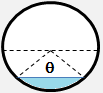
Analytical Functions for Circular Cross Sections
The following relation holds between the central angle θ (in radians) subtended by the water surface in the conduit's cross section (see figure above) and flow area A (French, 1985):
\[A = \frac{A_{full}(\theta - \sin\theta)}{2\pi}\]
Given a value for A, this expression is solved for θ using the following Newton-Raphson routine:
- Let \(\theta = 0.031715 - 12.79384\alpha + 8.28479\sqrt{\alpha}\) where \(\alpha = \frac{A}{A_{full}}\).
- Compute \(\Delta\theta = \frac{2\pi\alpha - (\theta - \sin\theta)}{(1 - \cos\theta)}\).
- Let \(\theta = \theta + \Delta\theta\).
- If \(|\Delta\theta| \leq 0.0001\) then stop. Otherwise return to step 2.
Once θ is known the remaining cross section variables can be found as follows:
Flow Depth: \(Y = Y_{full}\frac{(1 - \cos(\theta/2))}{2}\)
Section Factor: \(\Psi = \frac{\Psi_{full}(\theta - \sin\theta)^{5/3}}{(2\pi\theta^{2/3})}\)
Wetted Perimeter: \(P = \frac{\theta Y_{full}}{2}\)
Wetted Perimeter Derivative: \(P' = \frac{4}{Y_{full}(1 - \cos\theta)}\)
Hydraulic Radius: \(R = \frac{A}{P}\)
Section Factor Derivative: \(\Psi' = \left[\frac{5}{3} - \frac{2}{3}P'R\right]R^{2/3}\)
Figure 5-4 Ellipsoid and arch pipe cross sectional shapes
Figure 5-4 depicts standard ellipsoid and arch sewer pipe cross sectional shapes. Next to circular pipes these are the most commonly used shapes for newly installed sewers and culverts. Each shape is defined by its "rise" which is its full depth Yfull, and its "span" which is its maximum width Wmax. The vertical and horizontal ellipsoids have the same shape but rotated by 90 degrees (the span of one is the rise of the other and vice versa).
SWMM contains a list of 23 standard ellipsoid pipe sizes and 102 standard arch pipe sizes taken from the American Concrete Pipe Association's and the American Iron and Steel Institute's design manuals (American Concrete Pipe Association, 2011; American Iron and Steel Institute, 1999). The standard ellipsoid and arch pipe sizes are tabulated in Appendixes D and E, respectively. Each size is characterized by its rise, span, full area, and full hydraulic radius. Users can either select from one of these standard sizes or supply their own values for rise Yfull and span Wmax, both in feet. In the latter case the corresponding full area Afull and hydraulic radius Rfull are estimated using the formulas in Table 5-5.
Table 5-5 Full area and hydraulic radius of custom ellipsoid and arch pipe sections
| Property | Ellipsoid Shape | Arch Shape |
|---|---|---|
| Full Area \(A_{full}\) | \[1.2692Y_{full}^{2}\] | \[0.7879Y_{full}W_{\max}\] |
| Full Hydraulic Radius \(R_{full}\) | \[0.3061Y_{full}\] | \[0.2991Y_{full}\] |
Information in the aforementioned design manuals was used to construct the following tables for both the ellipsoid and arch shapes (only a single set of tables is needed for the two ellipsoid shapes since they are just rotated versions of one another):
| Atbl : | A/Afull as a function of Y/Yfull |
| Wtbl : | W/Wmax as a function of Y/Yfull |
| Rtbl : | R/Rfull as a function of Y/Yfull |
Each table contains entries for N = 26 equally spaced values of Y/Yfull between 0 and 1. The tables for ellipsoid pipes are in Appendix D and those for arch pipes are in Appendix E. To find A, W, or R for a given Y one first determines the integer portion of \((N - 1)\left( \frac{Y}{Y_{full}} \right)\), linearly interpolates the appropriate table between the entries at this and the next higher index, and then multiplies by the appropriate normalizing factor (either Afull, Wmax, or Rfull).
To find the depth associated with a given area Y(A), a bisection (or interval halving) procedure is first used on the appropriate (either ellipsoid or arch) area table Atbl to find the position i so that \(A_{tbl}\lbrack i\rbrack \leq \frac{A}{A_{full} \leq A_{tbl}\lbrack i + 1\rbrack}\). Then the desired depth Y is interpolated from this position in the table using the following expression with N = 26:
\[\Psi'(A) = \frac{\Psi(A + \Delta A) - \Psi(A - \Delta A)}{2\Delta A} \quad \text{where} \quad \Delta A = 0.001A_{full}\]
(5-15)
Figure 5-5 Masonry sewer shapes
SWMM contains seven pre-defined closed conduit shapes shown in Figure 5-5 that were used primarily in older masonry sewers built over a century ago. Their geometric properties have been derived from information and drawings found in Metcalf and Eddy (1914) and Davis (1952). These properties are represented using the same type of lookup tables discussed previously for circular cross sections (see section 5.2.3). The number of entries N in each table for each shape is listed in Table 5-6. The full tables are provided in Appendix F. The values of Afull, Rfull, and Wmax used to normalize the entries in the tables for each shape are listed in Table 5-7. The full section factor Ψfull used to normalize the section factor table is computed as \(A_{full}R_{full}^{2/3}\) .
Table 5-6 Number of entries in geometric property tables for masonry sewer shapes
| Shape | Atbl | Rtbl | Wtbl | Ytbl | Ψtbl |
|---|---|---|---|---|---|
| Basket Handle | 26 | 26 | 26 | 51 | 51 |
| Egg | 26 | 26 | 26 | 51 | 51 |
| Horseshoe | 26 | 26 | 26 | 51 | 51 |
| Catenary | — | — | 21 | 51 | 51 |
| Gothic | — | — | 21 | 51 | 51 |
| Semi-Circular | — | — | 21 | 51 | 51 |
| Semi-Elliptical | — | — | 21 | 51 | 51 |
Table 5-7 Geometric parameters of masonry sewer sections
| Shape | Afull | Rfull | Wmax | Ψmax |
|---|---|---|---|---|
| Basket Handle | \[0.7862Y_{full}^{2}\] | \[0.2464Y_{full}\] | \[0.944Y_{full}\] | \[1.06078\Psi_{full}\] |
| Egg | \[0.5105Y_{full}^{2}\] | \[0.1931Y_{full}\] | \[0.667Y_{full}\] | \[1.065\Psi_{full}\] |
| Horseshoe | \[0.8293Y_{full}^{2}\] | \[0.2538Y_{full}\] | \[Y_{full}\] | \[1.077\Psi_{full}\] |
| Catenary | \[0.70277Y_{full}^{2}\] | \[0.23172Y_{full}\] | \[0.9Y_{full}\] | \[1.05\Psi_{full}\] |
| Gothic | \[0.6554Y_{full}^{2}\] | \[0.2269Y_{full}\] | \[0.84Y_{full}\] | \[1.065\Psi_{full}\] |
| Semi-Circular | \[1.2697Y_{full}^{2}\] | \[0.2946Y_{full}\] | \[1.64Y_{full}\] | \[1.06637\Psi_{full}\] |
| Semi-Elliptical | \[0.785Y_{full}^{2}\] | \[0.242Y_{full}\] | \[Y_{full}\] | \[1.045\Psi_{full}\] |
The tables are used in the same manner as the ones for a circular shape to directly evaluate A(Y), W(Y), R(Y), Y(A), Ψ(A), and Ψ'(A). For the shapes that do not have an Atbl, A(Y) is determined using the inverse lookup method on the Ytbl described in section 5.2.4 for ellipsoids and arches. For shapes without an Rtbl, R(Y) is found by first finding A(Y) as just described, then finding Ψ(A) for the resulting area A, and finally evaluating \(\left( \frac{\Psi}{A} \right)^{3/2}\). Equation 5-15 is used to compute Ψ'(A).
Figure 5-6 shows four cross section shapes that are combinations of circular, rectangular, and triangular sections. The formulas for computing their geometrical properties are presented in the following paragraphs.
Figure 5-6 shows four cross section shapes that are combinations of circular, rectangular, and triangular sections. The formulas for computing their geometrical properties are presented in the following paragraphs.
Sediment Filled Circular Shape
This is a circular cross section that is partially filled with immobile sediment to a specified depth Ybtm. (This filled depth remains constant – SWMM does not model how it might change over time due to sediment transport processes.) The depth available for flow is \(Y_{full} - Y_{btm}\). To compute the geometric properties of this shape one first uses the circular shape functions to compute the area Abtm, top width Wbtm, and hydraulic radius R*btm* at a depth of Ybtm for the full circular shape with diameter Yfull. The wetted perimeter at this depth, Pbtm, is \(\frac{A_{btm}}{R_{btm}}\) . Then the expressions listed in Table 5-8 can be used to find the section properties for a specific flow depth Y above Ybtm or area A above Abtm .
Table 5-8 Geometric properties for a sediment filled circular cross section
| Property | Value Based on Full Circular Shape Functions |
|---|---|
| A(Y) | \[A\left( Y + Y_{btm} \right) - A_{btm}\] |
| W(Y) | \[W(Y + Y_{btm})\] |
| R(Y) | \[\frac{A\left( Y + Y_{btm} \right) - A_{btm}}{\left( \frac{A(Y + Y_{btm})}{R(Y + Y_{btm}}) \right) - P_{btm} + W_{btm}}\] |
| Y(A) | \[Y\left( A + A_{btm} \right) - Y_{btm}\] |
| Ψ(A) | \[A{R(\Delta Y)}^{2/3} \quad \text{where} \quad \Delta Y = Y\left( A + A_{btm} \right) - Y_{btm}\] |
| Ψ'(A) | \[\frac{\Psi(A + \Delta A) - \Psi(A - \Delta A)}{2\Delta A} \quad \text{where} \quad \Delta A = 0.001(A_{full} - A_{btm})\] |
Rectangular-Triangular Shape
This shape consists of a triangular bottom section of height Ybtm connected to a closed rectangular top section of width b and height Yfull – Ybtm. The slope of the triangular section's sidewalls s is \(\frac{b}{2Y_{btm}}\) . For depths below Ybtm (or areas below \(Y_{btm}\frac{b}{2}\)) the geometric properties are computed in the same manner as for the open triangular shape of section 5.2.1. At higher depths (or areas) the methods used for the closed rectangular shape of section 5.2.2 are applied with some adjustments made to accommodate the filled triangular section. The applicable formulas are listed in Table 5-9.
Table 5-9 Properties of the rectangular section of a rectangular-triangular shape
| Property | Expression |
|---|---|
| s | \[\frac{b}{\left( 2Y_{btm} \right)}\] |
\[A_{btm}\] | \[bY_{btm}/2\] |
\[A_{full}\] | \[b\left( Y_{full} - \frac{Y_{btm}}{2} \right)\] |
\[R_{full}\] | \[\frac{A_{full}}{\left( 2Y_{btm}\sqrt{1 + s^{2}} + 2\left( Y_{full} - Y_{btm} \right) + b \right)}\] |
\[\Psi_{full}\] | \[A_{full}R_{full}^{2/3}\] |
| A(Y) | \[A_{btm} + \left( Y - Y_{btm} \right)b\] |
| Y(A) | \[Y_{btm} + \frac{\left( A - A_{btm} \right)}{b}\] |
| W(Y) | \[b\] |
| P(Y) | \[2Y_{btm}\sqrt{\left( 1 + s^{2} \right)} + 2\left( Y - Y_{btm} \right)\] \[if\ \ A(Y) > 0.98A_{full}\ add\ on\ \left( \frac{A(Y)}{A_{full}} - 0.98 \right)\frac{b}{0.02}\ \ \] |
| R(Y) | \[\frac{A(Y)}{P(Y)}\] |
| R(A) | \[\frac{A}{P(Y(A))}\] |
\[\Psi_{\max}\] | \[0.98A_{full}{R(0.98A_{full})}^{2/3}\] |
\[\Psi(A)\] | \[A{R(A)}^{2/3}\ \ for\ A \leq 0.98A_{full}\] \[\Psi_{\max} + \left( \Psi_{full} - \Psi_{\max} \right)\frac{\left( \frac{A}{A_{full} - 0.98} \right)}{0.02\ \ for\ A > 0.98A_{full}}\] |
\[\Psi'(A)\] | \[\left( \frac{5}{3} - \left( \frac{2}{3} \right)\left( \frac{2}{b} \right)R(A) \right){R(A)}^{2/3}\ \ for\ A \leq 0.98A_{full}\] \[\frac{\left( \Psi_{full} - \Psi_{\max} \right)}{0.02A_{full}\ for\ A > 0.98A_{full}\ }\] |
Rectangular-Round Shape
This composite shape consists of a closed rectangular top with a rounded bottom section. It has full height Yfull, top width b, and bottom radius of curvature r (see Figure 5-6). Table 5-10 lists the parameters used to compute the section's properties whose formulas are given in Table 5-11.
Table 5-10 Geometric parameters for rectangular-round shapes
| Parameter | Value |
|---|---|
| Central Angle θ | \[2\sin^{- 1}\left( \frac{b}{2r} \right)\] |
| Bottom Section Height Ybtm | \[r\left( 1 - cos\left( \frac{\theta}{2} \right) \right)\] |
| Bottom Section Area Abtm | \[\left( \frac{r^{2}}{2} \right)\left( \theta - sin(\theta) \right)\] |
| Full Area Afull | \[b\left( Y_{full} - Y_{btm} \right) + A_{btm}\] |
| Full Hydraulic Radius Rfull | \[\frac{A_{full}}{\left\{ r\theta + 2\left( Y_{full} - Y_{btm} \right) + b \right\}}\] |
| Full Section Factor Ψfull | \[A_{full}R_{full}^{2/3}\] |
| Maximum Hydraulic Radius Rmax | \[\frac{0.98A_{full}}{\left\{ r\theta + \frac{2\left( 0.98A_{full} - A_{btm} \right)}{b} \right\}}\] |
| Maximum Section Factor Ψmax | \[0.98A_{full}R_{\max}^{2/3}\] |
Table 5-11 Geometric properties for rectangular–round shapes
| Property | Formula | Applicable Region |
|---|---|---|
| A(Y) | \[0.5r^{2}\left( \phi - \sin(\phi) \right) \quad \text{where} \quad \phi = 2\cos^{-1}\left( 1 - \frac{Y}{r} \right)\] | \[Y \leq Y_{btm}\] |
\[A_{btm} + \left( Y - Y_{btm} \right)b\] | \[Y > Y_{btm}\] | |
| W(Y) | \[2\sqrt{Y(2r - Y)}\] | \[Y \leq Y_{btm}\] |
| b | \[Y > Y_{btm}\] | |
| R(Y) | \[0.5r\frac{\left( 1 - \sin(\phi) \right)}{\phi} \quad \text{where} \quad \phi = 2\cos^{-1}\left( 1 - \frac{Y}{r} \right)\] | \[Y \leq Y_{btm}\] |
\[R\left( A(Y) \right) \quad \text{(see } R(A) \text{ function below)}\] | \[Y > Y_{btm}\] | |
| Y(A) | \[Y(A) \text{ for circular shape with } Y_{full} = 2r\] | \[A \leq A_{btm}\] |
\[Y_{btm} + \frac{\left( A - A_{btm} \right)}{b}\] | \[A > A_{btm}\] | |
| P(A) | \[2r\cos^{-1}\left( 1 - \frac{Y(A)}{r} \right)\] | \[A \leq A_{btm}\] |
\[2r\sin^{-1}\left( \frac{b}{2r} \right) + 2\frac{\left( A - A_{btm} \right)}{b}\] | \[A_{btm} < A \leq 0.98A_{full}\] | |
\[2r\sin^{-1}\left( \frac{b}{2r} \right) + 2\frac{\left( A - A_{btm} \right)}{b}\] \[+ \left( \frac{A}{A_{full} - 0.98} \right)\frac{b}{0.02}\] | \[A > 0.98A_{full}\] | |
| R(A) | \[\frac{A}{P(A)}\] | |
| Ψ(A) | \[\Psi(A) \text{ for circular shape with } Y_{full} = 2r\] | \[A \leq A_{btm}\] |
\[A{R(A)}^{2/3}\] | \[A_{btm} < A \leq 0.98A_{full}\] | |
\[\Psi_{\max} + \left( \Psi_{full} - \Psi_{\max} \right)\frac{\left( \frac{A}{A_{full} - 0.98} \right)}{0.02}\] | \[A > 0.98A_{full}\] | |
| Ψ'(A) | \[\frac{\left\{ \Psi(A + \Delta A) - \Psi(A - \Delta A) \right\}}{2\Delta A}\] | \[A \leq A_{btm}\] |
\[\left( \frac{5}{3} - \left( \frac{2}{3} \right)\left( \frac{2}{b} \right)R(A) \right){R(A)}^{2/3}\] | \[A_{btm} < A \leq 0.98A_{full}\] | |
\[\frac{\left( \Psi_{full} - \Psi_{\max} \right)}{\left( 0.02A_{full} \right)}\] | \[A > 0.98A_{full}\] |
Modified Basket Handle Shape
The modified basket handle shape is the reverse of the rectangular-round shape with a rectangular bottom section below a rounded top section. It has full height Yfull, bottom width b, and top section radius of curvature r (see Figure 5-6). The central angle θ formed by the rounded top section is:
\[\theta = 2\sin^{- 1}\left( \frac{b}{2r} \right)\]
(5-14)
The depth Ybtm of the bottom rectangular section is:
\[Y_{btm} = Y_{full} - r\left( 1 - cos\left( \frac{\theta}{2} \right) \right)\]
(5-15)
and its area Abtm is bYbtm . The shape's full area Afull is:
\[A_{full} = A_{btm} + \frac{r^{2}}{\left\{ 2(\theta - sin\theta) \right\}}\]
(5-16)
For depths up to Ybtm and areas up to Abtm the open rectangular shape functions of Tables 5-1 and 5-2, respectively, are used to compute the modified basket handle's section properties. For depths and areas above this the functions listed in Table 5-12 are used.
Table 5-12 Properties in the rounded top section of a modified basket handle shape
| Property | Expression |
|---|---|
| A(Y) | \[A_{full} - \left( \frac{r^{2}}{2} \right)(\phi - \sin\phi) \quad \text{where} \quad \phi = 2\cos^{-1}\left( 1 - \frac{\left( Y_{full} - Y \right)}{r} \right)\] |
| W(Y) | \[2\sqrt{\left( Y_{full} - Y \right)\left( 2r - \left( Y_{full} - Y \right) \right)}\] |
| R(Y) | \[R\left( A(Y) \right) \quad \text{using } R(A) \text{ function below}\] |
| Y(A) | \[Y_{full} - Y\left( A_{full} - A \right) \quad \text{using } Y(A) \text{ for circular shape with } Y_{full} = 2r\] |
| P(A) | \[(\theta - \phi)r + 2\left( Y_{full} - Y(A) \right) + b \quad \text{where} \quad \phi = 2\cos^{-1}\left( 1 - \frac{\left( Y_{full} - Y(A) \right)}{r} \right)\] |
| R(A) | \[\frac{A}{P(A)}\] |
\[\Psi(A)\] | \[A{R(A)}^{2/3}\] |
\[\Psi'(A)\] | \[\frac{\left\{ \Psi(A + \Delta A) - \Psi(A - \Delta A) \right\}}{(2\Delta A)} \quad \text{where} \quad \Delta A = 0.001A_{full}\] |
The solution method for kinematic wave analysis in a closed conduit needs to know what cross-sectional area corresponds to the flow depth where the section factor and hence the Manning equation flow rate is a maximum (see Sections 4.2 and 4.3.2). Below this point the section factor is an increasing function of area, after which it decreases until the conduit becomes full. Table 5-13 lists the ratio of the area at maximum flow (denoted as Amax) to the full area (Afull) for the standard closed conduit shapes recognized by SWMM. For open shapes Amax is the same as Afull.
Table 5-13 Area at maximum flow to full area for standard closed conduits shapes
| Shape | \[\frac{\mathbf{A}_{\mathbf{\max}}}{\mathbf{A}_{\mathbf{full}}}\] | Shape | \[\frac{\mathbf{A}_{\mathbf{\max}}}{\mathbf{A}_{\mathbf{full}}}\] |
|---|---|---|---|
| Rectangular | 0.97 | Circular | 0.9756 |
| Elliptical | 0.96 | Arch | 0.92 |
| Basket Handle | 0.96 | Egg | 0.96 |
| Horseshoe | 0.96 | Catenary | 0.98 |
| Gothic | 0.96 | Semi-Circular | 0.96 |
| Semi-Elliptical | 0.98 | Rectangular-Triangular | 0.98 |
| Rectangular-Round | 0.98 | Modified Basket Handle | 0.96 |
Kinematic wave analysis also needs to know the area A corresponding to a given normal flow rate Q from its associated section factor Ψ, where \(\Psi = \frac{Q\sqrt{S_{0}}}{\eta}\). For circular shapes and the seven masonry sewer shapes discussed in section 5.2.5 the following "reverse" lookup method is used with the shape's Ψ versus A table (Ψtbl) to determine A given Ψ.
Let Ψ* be the section factor value whose area is sought and let N be the number of entries in Ψtbl. First the interval in the table that brackets \(\frac{\Psi^{*}}{\Psi_{full}}\) is located. Since these are all closed shapes, there will be a table entry index imax after which the \(\frac{\Psi}{\Psi_{full}}\) values begin to decrease. If \(\frac{\Psi^{*}}{\Psi_{full}}\) is between Ψtbl[imax] and Ψtbl[N] then this portion of the table is examined to find the index i* so that \(\frac{\Psi^{*}}{\Psi_{full}}\) is between Ψtbl[i*] and Ψtbl[i*+1]. Otherwise a bisection search is used between index 0 and imax to find the interval starting at i* that brackets \(\frac{\Psi^{*}}{\Psi_{full}}\). Then the area A* corresponding to Ψ* is computed as:
\[A^{*} = \frac{A_{full}}{(N - 1)}\left( i^{*} + \frac{\left( \Psi^{*} - \Psi_{tbl}\left\lbrack i^{*} \right\rbrack \right)}{\left( \Psi_{tbl}\left\lbrack i^{*} + 1 \right\rbrack - \Psi_{tbl}\left\lbrack i^{*} \right\rbrack \right)} \right)\]
(5-17)
For all other shapes the Newton-Raphson-Bisection method (see Appendix A) is used to find the solution of
\(f(A) = \Psi(A) - \Psi^{*} = 0\) (5-18)
where Ψ* is the section factor value whose corresponding area is sought. The derivative of f(A) required by the method is the shape's Ψ'(A) function. If the shape is closed with Amax < Afull and Ψ* is between Ψfull and Ψmax then the search interval is [Afull, Amax]. Otherwise it is [0, Amax]. The convergence criterion is 0.01 percent of Afull .
In addition to its catalog of standard pre-defined shapes, SWMM can also utilize custom closed shapes that are defined by a Shape Curve supplied by the user. This curve specifies how the width of the cross-section varies with height, where both width and height are scaled relative to the section\'s full height. This allows the same shape curve to be used for conduits of differing sizes. An example shape curve along with its table of width versus height is shown in Figure 5-7.
|
|
Figure 5-7 A Shape Curve with a depth segment shown
The flow area A, top width W and hydraulic radius R of a custom shape are pre-computed at 51 equally spaced vertical values between 0 and 1 along the shape curve and stored in tables Atbl, Wtbl, and Rtbl, respectively. The tables are constructed by analyzing each depth segment of size 1/50 = 0.02 starting at 0 and working upwards. As shown in Figure 5-7, each depth segment forms a trapezoid within the cross section. The area of this trapezoid is added to the shape's total area Asum and the length of its side walls is added to the total wetted perimeter Psum. If the depth segment straddles more than one shape curve segment, then additional trapezoids are formed at the shape curve's vertices, each of which contributes to Asum and Psum. The Atbl entry for the segment is set to Asum, the Rtbl entry to \(\frac{A_{sum}}{P_{sum}}\), and the Wtbl entry to the segment's top width.
When a conduit with full depth Yfull is assigned a shape curve for its cross section, the curve's geometry tables are used in the same manner as the tables for ellipsoid and arch shapes described in section 5.1.4 for evaluating A(Y), W(Y), R(Y), Y(A), Ψ(A), and Ψ'(A). The values of Afull, Rfull, and Wmax used to convert the normalized values in the tables to actual dimensions are as follows:
\[A_{full} = A_{tbl}\lbrack 50\rbrack Y_{full}^{2}\]
(5-19)
\[R_{full} = R_{tbl}\lbrack 50\rbrack Y_{full}\]
(5-20)
\[W_{\max} = \left\{ \max_{0 \leq i \leq 50}{W_{tbl}\lbrack i\rbrack} \right\} Y_{full}\]
(5-21)
The value of Amax, the area of the flow depth where the section factor is a maximum, is given by:
\[A_{\max} = \left\{ \max_{0 \leq i \leq 50}\left( A_{tbl}\lbrack i\rbrack{R_{tbl}\lbrack i\rbrack}^{2/3} \right) \right\} Y_{full}^{2}\]
(5-22)
The Newton-Raphson-Bisection method described in section 5.1.8 is used to evaluate A(Ψ).
Figure 5-8 A natural channel transect
SWMM also has the ability to model natural channels with irregular shaped cross sections. The cross sectional shape is represented by a transect that begins at the top of the left bank of the channel (looking downstream) and extends transversely across the channel to the top of its right bank. The channel's bed elevation (y) relative to a known elevation is recorded at a series of measurement stations (x) across the transect (see Figure 5-8). A single transect is used to represent a channel's cross section along its entire length. This might require that longer channels with varying cross section profiles be broken into smaller more uniform segments.
As shown in Figure 5-8, transects can contain two overbank areas on either side. Each is optional and is used to specify a different Manning's roughness coefficient than that assigned to the main channel. Each overbank boundary location must coincide with one of the transect's measurement stations.
The flow area A, top width W and hydraulic radius R of a transect are pre-computed at 51 equally spaced values of flow depth relative to full depth \(\left( \frac{Y}{Y_{full}} \right)\) and stored in tables Atbl, Wtbl, and Rtbl, respectively. The table values are normalized with respect to the full section area A*full, the maximum width *Wmax, and the full section hydraulic radius Rfull, respectively. These tables are used in the same manner as the tables for ellipsoid and arch shapes described in section 5.1.4 for evaluating A(Y), W(Y), R(Y), Y(A), Ψ(A), and Ψ'(A). A(Ψ) is found using the Newton-Raphson-Bisection method as described in section 5.1.8.
The first step in constructing the geometric property tables for a transect is to find the measurement stations with the lowest and highest elevations. The full channel depth Yfull is set equal to the difference between these values. If necessary, a new station is added at either end of the transect so that both ends are at the highest elevation. Then all station elevation values y are converted to the height above the lowest elevation station.
Next table entries are generated for a series of depths that divide the full depth into 50 equal increments starting at 0 (whose table entries are set to 0). The procedure for finding each table's entry for the k-th depth interval is described in the side bar entitled "*Computing Geometry Table Entries for Irregular Cross Sections*". It traverses the cross section's transect, computing the area, width, and wetted perimeter for each measurement station segment that lays above the current depth increment. It also finds the conductance (the section factor times roughness) of compound segments that separate regions of differing roughness or where valleys occur in the transect's profile. (Figure 5-9 shows a flow depth increment with three compound segments.) After the end of the transect is reached the sum of the compound conductances is used along with the main channel roughness to find the hydraulic radius for the current depth increment.
Figure 5-9 A transect depth increment with three compound segments
Once table entries for all depth increments have been generated, the following quantities are assigned and used to normalize the entries in their respective tables: \(A_{full} = A_{tbl}[50]\), \(W_{\max} = W_{tbl}[50]\), \(R_{full} = R_{tbl}[50]\). Another adjustment is to set Wtbl[0] = Wtbl[1] since the above procedure does not calculate a width at zero depth.
Computing Geometry Table Entries for Irregular Cross Sections
To find the k-th entry in an irregular cross section's geometry tables first initialize the following:
Flow depth: \(Y = k\frac{Y_{full}}{50}\)
Table entries for index k: \(A_{tbl}[k] = 0\), \(W_{tbl}[k] = 0\), \(R_{tbl}[k] = 0\)
Compound segment area: \(A_{sum} = 0\)
Compound wetted perimeter: \(P_{sum} = 0\)
Total flow conductance: \(K = 0\)
Transect station index: \(i = 1\)
- Select the cross section segment between transect stations at \(x_{i-1}\) and \(x_i\).
- If the flow depth is below the channel bottom ( \(Y < \min(y_{i-1}, y_i)\)) go to step 10.
- Compute the width \(w\) and wetted perimeter \(p\) of the full segment:
\[w = x_i - x_{i-1}\]
\[p = \sqrt{w^2 + \Delta y^2} \quad \text{where} \quad \Delta y = |y_i - y_{i-1}|\]
- If the segment is completely submerged ( \(Y > \max(y_{i-1}, y_i)\)) compute its area \(a\) as:
\[a = w\left(Y - \frac{(y_{i-1} + y_i)}{2}\right)\]
Otherwise let \(\alpha = \frac{(Y - \min(y_{i-1}, y_i))}{\Delta y}\) and set \(a = \frac{\alpha^2 w\Delta y}{2}\).- Adjust the width and wetted perimeter for partial submergence:
\[w = \alpha w; \quad p = \alpha p\]
- Update the table entries for area and top width:
\[A_{tbl}[k] = A_{tbl}[k] + a; \quad W_{tbl}[k] = W_{tbl}[k] + w\]
- Update the area and wetted perimeter of the current compound segment:
\[A_{sum} = A_{sum} + a; \quad P_{sum} = P_{sum} + p\]
- Let \(n_i\) be the roughness coefficient between stations \(i-1\) and \(i\). If station \(i\) marks the end of a compound segment ( \(y_i > Y\) or \(n_i \neq n_{i+1}\)) then update the total conductance:
\[K = K + \frac{1.486}{n_i}A_{sum}\left(\frac{A_{sum}}{P_{sum}}\right)^{2/3}\]
and begin a new compound segment by setting \(A_{sum}\) and \(P_{sum}\) to 0.- If more transect stations remain, increment the station index, \(i = i + 1\) and go to Step 2.
- Compute the hydraulic radius table entry:
\[R_{tbl}[k] = \left(\frac{n_C K}{1.486A_{tbl}[k]}\right)^{3/2}\]
where \(n_C\) is the main channel roughness.
An irregular natural channel can also be assigned a meander modifier. This is the ratio of the length of a meandering main channel to the length of the overbank area that surrounds it. While the user-supplied length for the overall channel is that of the longer main channel, SWMM will use the shorter overbank length in its calculations. The Manning's n of the main channel will be increased by the square root of the meander modifier to provide an equivalent friction head loss over the reduced main channel length.
SWMM defines the geometry of a street or roadway cross-section as a special case of the irregular channel discussed in the previous section. The shape of a one-sided street cross-section is shown in Figure 5-10. In its most basic form it consists of a road surface with downward slope Sx extending a distance of Tcrown to a vertical curb of height Hcurb. To this can be added:
A two sided street cross-section adds a mirror image of the one-sided street to the right of the street crown with the same roadway, gutter, curb, and backing dimensions.
Figure 5-10 A one-sided street cross-section (not to scale)
Street cross-sections use the same procedures as irregular channel transects, described in section 5.3, to compute tables of flow area, top width, and hydraulic radius at 50 equally spaced increments of flow depth (for both one-sided and two-sided streets). This requires that in addition to the dimensions shown in Figure 5-10, a Manning roughness coefficient must be specified for the road surface and for the backing surface if present.
SWMM's hydraulic modeling procedures require knowledge of how a storage unit's surface area A and volume V vary with surface depth Y above the bottom of the unit. It is sufficient to specify either an area or volume relationship with respect to depth since one can be derived from the other \(\left( A = \frac{dV}{dY} \text{ and } V = \int AdY \right)\). SWMM uses surface area to describe a storage unit's shape. One can select either from several standard shapes where A is a quadratic function of Y, from a general power law relation between A and Y or use a tabular listing of Y and A values.
SWMM supports several common storage unit shapes, listed in Table 5-14, whose top surface area A can be expressed as a quadratic function of height Y:
\[A = a_{0} + a_{1}Y + a_{2}Y^{2}\]
(5-23)
The constants a0, a1, and a2 depend on the shape's dimensions as shown in Table 5-14.
Table 5-14. Standard storage unit shapes.
| Shape | Coefficients | Dimensions | |
|---|---|---|---|
| Elliptical Cylinder |
| \[a_{0} = \left( \frac{\pi}{4} \right)LW\] \[a_{1} = a_{2} = 0\] | L = major axis length W = minor axis width |
| Elliptical Paraboloid |
| \[a_{0} = a_{2} = 0\] \[a_{1} = (\frac{\pi}{4})\frac{LW}{H}\] | L = major axis length W = minor axis width H = paraboloid height |
| Elliptical Cone |
| \[a_{0} = \left( \frac{\pi}{4} \right)LW\] \[a_{1} = \pi WZ\] \[a_{2} = \pi(\frac{W}{L})Z^{2}\] | L = bottom major axis length W = bottom minor axis width Z = side slope (run/rise) along major axis |
| Rectangular Pyramid |
| \[a_{0} = LW\] \[a_{1} = 2(L + W)Z\] \[a_{2} = 4Z^{2}\] | L = bottom length W = bottom width Z = wall slope (run/rise) (same for each face) |
Dynamic wave analysis needs to know how volume V varies with depth Y. Integrating Equation 5-23 over depth yields:
\[V = a_{0}Y + \frac{a_{1}}{2}Y^{2} + \frac{a_{2}}{3}Y^{3}\]
(5-24)
Kinematic wave analysis needs to know the depth associated with a given volume. For a cylindrical shape: \(Y = V/a_{0}\), while for paraboloid shape: \(Y = \sqrt{2V/a_{1}}\) . For the other shapes the cubic equation 5-24 is solved numerically for Y given V using the Newton-Raphson-Bisection method described in Appendix A over the interval [0, Yfull] with initial estimate \(Y = \frac{V}{a_{0}},\) convergence tolerance of 0.001 ft and derivative given by Equation 5-23.
The four standard shapes are declared in the [STORAGE] input section with the keywords CYLINDRICAL, CONICAL, PARABOLIC (the alias PARABOLOID is also accepted on input) and PYRAMIDAL, each followed by the three dimensions listed in Table 5-14 in the order shown (the elliptical cylinder's third dimension is unused). The dimensions must satisfy L > 0 and W > 0, with Z ≥ 0 for the cone and pyramid and H > 0 for the paraboloid; the quadratic coefficients a0, a1 and a2 are derived from them internally. The raw dimensions are retained alongside the derived coefficients so that a model written back to file reproduces the shape and its dimensions exactly rather than a functional equivalent. If a node is assigned both a storage curve (Section 5.5.3) and a shape, the curve takes precedence.
Implementation. The dimension validation and the coefficient formulas of Table 5-14 are defined in one place, src/engine/data/StorageGeometry.hpp (storage_shape_coeffs), shared by the [STORAGE] parser (src/engine/input/handlers/NodesHandler.cpp), the input writer and the editing API. The quadratic area relation 5-23, its cubic volume integral 5-24 and the closed-form and Newton depth inversions are evaluated in src/engine/hydraulics/Node.cpp.
SWMM's functional storage shape option uses a power law to relate surface area to depth:
\[A = c_{0} + c_{1}Y^{c_{2}}\]
(5-25)
where c0, c1, and c2 are user-supplied constants.
The surface area at a given depth is found directly from this equation. The relation between volume V and depth Y (required for dynamic wave analysis) is:
\[V = c_{0}Y + \left( \frac{c_{1}}{c_{2} + 1} \right)Y^{c_{2} + 1}\]
(5-26)
To find the depth associated with a given volume (required for kinematic wave analysis) one solves the following nonlinear equation for Y :
\[f(Y) = V - \left( c_{0}Y + \left( \frac{c_{1}}{c_{2} + 1} \right)Y^{c_{2} + 1} \right) = 0\]
(5-27)
It is solved using the Newton-Raphson-Bisection method described in Appendix A over the interval [0, Yfull] with initial estimate \(Y = \frac{V}{\left( c_{0} + c_{1} \right)},\) convergence tolerance of 0.001 ft and derivative \(f'(Y)\) given by Equation 5-25.
Some shapes and their coefficients that can be represented with this functional option include:
c0 = area of the base
c1 = c2 = 0.
An open channel with a trapezoidal cross section and vertical ends:
\[c_{0} = WL\]
\[c_{1} = 2ZL\]
\[c_{2} = 1\]
where W = bottom width of cross section, L = channel length, and Z = side slope.
An open channel with a parabolic cross section and vertical ends:
\[c_{0} = 0\]
\[c_{1} = WLH^{0.5}\]
\[c_{2} = 1\]
where W = top width, L = channel length and H = full height.
An elliptical paraboloid:
\[c_{0} = 0\]
\[c_{1} = A/H\]
\[c_{2} = 1\]
where A is the surface area at height H.
The shape of a storage unit can also be defined by a Storage Curve which is a series of user-supplied data pairs Yi, Ai that represent the points on a curve of surface area versus surface depth for the unit. An example of this type of curve is shown in Figure 5-11. It can represent natural depressions with irregular shaped contour intervals, spheroid storage vessels or conventional shapes with different base sizes stacked on top of one another. The first point supplied to the curve should be the surface area of the unit\'s base at a depth of 0. Otherwise it will be assumed that the unit has zero surface area at its base. The curve will be extrapolated outwards to meet the unit\'s maximum depth if need be.
Figure 5-11 Example of a storage curve and its section view
To find the area associated with a given storage depth one interpolates between the data points that bracket the depth value on the storage curve. Determining the storage volume V at a given depth Y is equivalent to finding the area under the storage curve from depth 0 to Y. This can be done by using the Trapezoidal Rule (Atkinson, 1989) which results in:
\[V = \frac{1}{2}\left\{ \sum_{i = 1}^{n}{\left( Y_{i} - Y_{i - 1} \right)\left( A_{i} + A_{i - 1} \right)} \right\} + \frac{1}{2}\left( Y - Y_{n} \right)\left( A + A_{n} \right)\]
(5-28)
where n is the largest data point index with \(Y_{n} \leq Y\) and A is the surface area associated with depth Y as found from the storage curve itself. The shaded rectangles in Figure 5-12 illustrate how the trapezoidal rule is applied to a storage curve to find the stored volume at a particular depth. This procedure is the same as the widely used Average-End-Area method except that the area at the desired depth is first interpolated from the storage curve rather than converting the original area curve to a volume curve and interpolating directly from it.
Figure 5-12 Finding the volume at a given depth for a storage curve
The depth that corresponds to a particular volume for a storage curve can be found as follows. Using the trapezoidal rule, sum the volumes contributed by each curve segment starting from 0 until the accumulated volume Vsum exceeds the target volume V. Let the data point index at the start of this segment be denoted by i. Then the depth Y that results in volume V is:
\[Y = Y_{i} + \frac{\left\lbrack \sqrt{A_{i}^{2} + 2\alpha\left( V - V_{sum} \right)} - A_{i} \right\rbrack}{\alpha}\]
where \(\alpha = \frac{\left( A_{i + 1} - A_{i} \right)}{\left( Y_{i + 1} - Y_{i} \right)}\). (5-29)
SWMM needs to calculate the critical and normal flow depths in a conduit for dynamic wave analysis whenever:
These depths are functions of flow rate and cross section shape. For all but the simplest shapes, iterative numerical methods are required to compute them.
Critical depth is defined as the depth Y where the specific energy at a given flow rate Q is a minimum and the Froude number Fr equals 1 (Chow, 1959). From the latter condition
\[Fr = \frac{U}{\sqrt{g\frac{A}{W}}} = 1\]
(5-30)
where U is flow velocity and g is the acceleration of gravity. Since \(U = \frac{Q}{A}\) and both area and width are functions of flow depth, at the critical flow depth YC the following relation holds:
\[\frac{{A\left( Y_{C} \right)}^{3}}{W\left( Y_{C} \right)} = \frac{Q^{2}}{g}\]
(5-31)
YC can be computed explicitly for several simple conduit shapes. The formulas are listed in Table 5-14. Other shapes require that an iterative root finding procedure be applied to the following re-arranged form of Equation 5-29:
\[f(Y) = \frac{{A(Y)}^{3}}{W(Y)} - \frac{Q^{2}}{g} = 0\]
(5-32)
Because analytical derivatives of f(Y) are not available for most shapes, derivative-free methods are used instead of the Newton-Raphson method. Two such methods are interval enumeration and Ridder's method (Press et al., 1992). Ridder's method is a variation on the method of false position. The user supplies a set of depths Y1 and Y2 that bracket YC along with a stopping tolerance ε. The full algorithm is described in Appendix B.
Table 5-14 Critical depth formulas for simple section shapes
| Shape | Formula | Remarks |
|---|---|---|
| Rectangular1 | \[Y_{C} = \left( \frac{Q^{2}}{gb^{2}} \right)^{1/3}\] | b = width |
| Triangular1 | \[Y_{C} = \left( \frac{2Q^{2}}{gs^{2}} \right)^{1/5}\] | s = side slope |
| Parabolic2 | \[Y_{C} = \left( \frac{27\alpha Q^{2}}{32g} \right)^{1/4}\] | Perimeter Equation: \(y = \alpha x^{2}\) |
| Power Law2 | \[Y_{C} = \left( \frac{(1 + \gamma)^{3}\alpha^{2\gamma}Q^{2}}{4g} \right)^{\frac{1}{(3 + 2\gamma)}}\] | Perimeter Equation: \(y = \alpha x^{\frac{1}{\gamma}}\) |
1French (1985).
2Swamee (1993).
With interval enumeration the full depth of the cross section is divided into N equal intervals (SWMM 5 currently uses N = 25). Given a flow Q and an initial estimate of its critical depth YC, the following steps are used to calculate its actual value:
If \(Q_{0} < Q\):
a. Set \(i = i + 1\), \(Y = i\frac{Y_{full}}{N}\), and \(Q_{C} = \sqrt{g\frac{{A(Y)}^{3}}{W(Y)}}\).
b. If \(Q_{C} \geq Q\) then stop with \(Y_{C} = \left\lbrack \frac{\left( Q - Q_{0} \right)}{\left( Q_{C} - Q_{0} \right) + (i - 1)} \right\rbrack\left( \frac{Y_{full}}{N} \right)\).
c. Set \(Q_{0} = Q_{C}\) and go to step a.
Otherwise:
a. Set \(i = i - 1\), \(Y = i\frac{Y_{full}}{N}\), and \(Q_{C} = \sqrt{g\frac{{A(Y)}^{3}}{W(Y)}}\).
b. If \(Q_{C} < Q\) then stop with \(Y_{C} = \left\lbrack \frac{\left( Q - Q_{C} \right)}{\left( Q_{0} - Q_{C} \right) + i} \right\rbrack\left( \frac{Y_{full}}{N} \right)\).
c. Set \(Q_{0} = Q_{C}\) and go to step a.
Empirical testing has shown that the interval enumeration method tends to use less iterations than Ridder's method when:
The initial estimate of YC is computed from the following approximation for circular sections (French 1985):
\[Y_{C} = 1.01\frac{\left( \frac{Q^{2}}{g} \right)^{0.25}}{Y_{full}^{0.26}}\]
(5-33)
Therefore interval enumeration is used when the first condition listed above holds, with the second condition used to set the initial estimate of YC. Otherwise Ridder's method is used with Equation 5-30 as the function whose root YC is to be found with a convergence tolerance of 0.001 feet. The initial bracket [Y1 , Y2] on YC is determined as follows:
If \(Q_{0} > Q\) then:
a. Set \(Y_{2} = Y_{0}\).
b. If \(Q_{1/2} < Q\) then set \(Y_{1} = Y_{1/2}\), otherwise set \(Y_{1} = 0\).
Otherwise:
a. Set \(Y_{1} = Y_{0}\).
b. If \(Q_{1/2} > Q\) then set \(Y_{2} = Y_{1/2}\), otherwise set \(Y_{2} = 0.99Y_{full}\).
Normal depth is defined as the flow depth that results in a given uniform flow rate along a conduit. When the Manning equation is used to describe uniform flow, the relation between flow rate Q and normal depth YN is:
\[A(Y_{N}){R(Y_{N})}^{2/3} = \frac{Q\eta}{\sqrt{S_{0}}}\]
(5-34)
where η is the Manning roughness expressed in US units and S0 is the conduit's slope. From the definition of the section factor Ψ introduced in Chapter 4, Equation 5-34 can be written as:
\[\Psi = \frac{Q\eta}{\sqrt{S_{0}}}\]
(5-35)
To find YN for flow rate Q one first computes Ψ from Equation 5-35, then finds the flow area A that produces this value of Ψ using the methods described in section 5.1.8 and finally evaluates the depth that produces this area using the Y(A) function for the particular shape being analyzed. In equation terms:
\[Y_{N} = Y\left( A\left( \Psi = \frac{Q\eta}{\sqrt{S_{0}}} \right) \right)\]
(5-36)
 1.13.2