The kinematic wave model is derived from a simplified form of the St. Venant equations that combines the continuity equation with the uniform flow equation. It cannot model pressurized flow, reverse flow, or backwater effects. It is most applicable to steeply sloped conduits subjected to long duration inflow hydrographs that produce shallow flow with high velocity (Ponce et al., 1978). For these situations its results will not be far off from those of dynamic wave analysis and can be computed much more efficiently using much larger time steps.

Kinematic wave modeling was included in the original release of SWMM in 1971 before a full dynamic wave option was available. The original method included an enhancement to approximate a backwater effect for sub-critical flow. SWMM 5 has dropped this enhancement in favor of the classical kinematic wave formulation since the code now includes a full dynamic wave option (described in the previous chapter) that rigorously models backwater effects.

4.1 Governing Equations

The kinematic wave model for unsteady flow in a channel or pipe is derived from the same St. Venant equations for conservation of mass and momentum that were used for dynamic wave analysis:


\[\frac{\partial A}{\partial t} + \frac{\partial Q}{\partial x} = 0\]	Continuity	(4-1)
\[\frac{\partial Q}{\partial t} + \frac{\partial\left( \frac{Q^{2}}{A} \right)}{\partial x} + gA\frac{\partial H}{\partial x} + gAS_{f} = 0\]	Momentum	(4-2)

where all variables were defined previously in Chapter 3. Expressing head H as Z + Y (invert elevation plus flow depth) and recognizing that \(\frac{\partial Z}{\partial x} = -S_{0}\) (the conduit's slope) allows one to write the momentum equation as:

\[\frac{\partial Q}{\partial t} + \frac{\partial\left( \frac{Q^{2}}{A} \right)}{\partial x} + gA\frac{\partial Y}{\partial x} = gA(S_{0} - S_{f})\]

(4-3)

If one assumes that the terms on the left hand side of Equation 4-3 are negligible one is left with the relation:

\[S_{0} = S_{f}\]

(4-4)

Having the conduit's bottom slope equal the friction slope implies that the fluid motion caused by gravity is balanced by the frictional resistance to flow. Using the Manning equation to represent the friction slope allows one to represent the relationship between flow rate Q and flow area A with Manning's equation for steady uniform flow:

\[Q = \frac{AR^{2/3}\sqrt{S_{0}}}{\eta}\]

(4-5)

where the hydraulic radius R is an implicit function of flow area A for a specific conduit cross-sectional shape. (R is defined as area divided by wetted perimeter where the latter can be determined from flow depth which can be inferred from the flow area A.)

By defining \(\beta = \frac{\sqrt{S_{0}}}{\eta}\) and \(\Psi = AR^{2/3}\) the Manning equation can be expressed as:

\[Q = \beta\Psi(A)\]

(4-6)

Ψ is known as the section factor (Chow, 1959) and is a function of the flow area and conduit geometry. For some closed conduit shapes, such as circular pipes, the section factor achieves a maximum value at a less than full flow area (as shown in Figure 4-1) resulting in a maximum flow that is larger than when the conduit flows full.

figure4-1.png

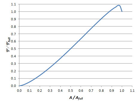
Figure 4-1 Section factor versus area for a circular shape

Thus the governing equations for kinematic wave modeling along a single conduit are the continuity equation 4-1 along with the "rating curve" equation 4-6 that relates flow rate to area. The dependent variables in these equations are flow rate Q and flow area A, which are functions of distance x and time t. To solve these equations over a single conduit of length L, one needs a set of initial conditions for either Q or A at time 0 as well as boundary condition for either variable at x = 0 for all times t.

4.2 Solution Method

The material that follows applies to networks containing only conduits connected by junction nodes, where there is at most one outflow conduit from each junction. Inclusion of flow control devices (pumps, orifices, and weirs) and other processes (seepage and evaporation) will be covered in subsequent chapters of this manual. Allowances for both flow divider nodes and storage nodes are discussed later in this chapter in Section 4.3.

The continuity equation 4-1 is solved along a space-time grid depicted in Figure 4-2. A weighted Wendroff implicit finite difference scheme (Smith, 1978) is used to re-express the equation as:

\[\frac{(1 - \theta)\left( A_{1}^{t + \Delta t} - A_{1}^{t} \right) + \theta\left( A_{2}^{t + \Delta t} - A_{2}^{t} \right)}{\Delta t} + \frac{(1 - \phi)\left( Q_{2}^{t} - Q_{1}^{t} \right) + \phi\left( Q_{2}^{t + \Delta t} - Q_{1}^{t + \Delta t} \right)}{L} = 0\]

(4-7)

image20

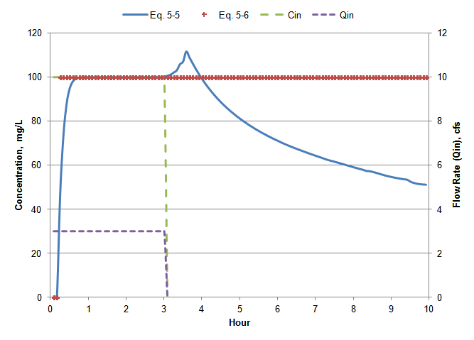
Figure 4-2 Space-time grid for kinematic wave analysis

The subscripts 1 and 2 on A and Q refer to the upstream and downstream ends of the conduit, respectively. The superscript refers to the time period. θ and φ are weights chosen to be between 0.5 and 1. At each time step this equation is applied conduit by conduit starting at the most upstream node and working downstream. The only unknowns will be \(A_{2}^{t + \Delta t}\) and \(Q_{2}^{t + \Delta t}\). As there is only one outflow conduit connected to a junction node, \(Q_{1}^{t + \Delta t}\) is known from the sum of the already computed \(Q_{2}^{t + \Delta t}\) values of the upstream conduits that flow into the conduit being analyzed, and also includes any externally imposed inflows such as wet weather runoff or dry weather sanitary flow. The area \(A_{1}^{t + \Delta t}\) associated with this flow can be found by evaluating the inverse of the section factor at the value of \(\frac{Q_{1}^{t + \Delta t}}{\beta}\).

The Manning equation 4-6 can be substituted into Equation 4-7 which after some rearrangement results in the following nonlinear equation with single unknown \(A_{2}^{t + \Delta t}\):

\[f\left( A_{2}^{t + \Delta t} \right) = \beta\Psi\left( A_{2}^{t + \Delta t} \right) + C1A_{2}^{t + \Delta t} + C2 = 0\]

(4-8)

where the constants C1 and C2 are given by:

\[C1 = \frac{L\theta}{\Delta t\phi}\]

(4-9)

\[C2 = \frac{L}{\Delta t\phi}\left\lbrack (1 - \theta)\left( A_{1}^{t + \Delta t} - A_{1}^{t} \right) - \theta A_{2}^{t} \right\rbrack + \frac{1 - \phi}{\phi}\left( Q_{2}^{t} - Q_{1}^{t} \right) - Q_{1}^{t + \Delta t}\]

(4-10)

After solving 4-8 for \(A_{2}^{t + \Delta t}\) equation 4-6 can then be used to find the corresponding flow \(Q_{2}^{t + \Delta t}\).

Equation 4-8 is solved using a combination of bisection and Newton-Raphson methods (Press et al., 1992) with both θ and φ set to 0.6. As a first step, a bracket \(\left\lbrack A_{LOW},\ A_{HIGH} \right\rbrack\) is sought where \(f(A_{LOW})\) and \(f(A_{HIGH})\) are of opposite sign. For conduit shapes whose section factor has a maximum value at an area A_max below A_full (such as the circular conduit of Figure 4-1), these two areas are tried first. If these areas do not form a valid bracket then 0 to A_max is used. For shapes whose section factor always increases with increasing area, 0 to A_full is used.

If a valid bracket is found then the procedure described in Appendix A, "*Newton-Raphson-Bisection Root Finding Method*", is used to find \(A_{2}^{t + \Delta t}\). Its initial estimate is \(A_{2}^{t}\) and a convergence tolerance ε of 0.1 percent of A_full is used. The derivative of f(A) required by the method is \(f'(A) = \beta\Psi'(A) + C1\) where \(\Psi'(A)\) is the derivative of the section factor with respect to area A. If \(\left\lbrack A_{LOW},\ A_{HIGH} \right\rbrack\) does not form a valid bracket then \(A_{2}^{t + \Delta t}\) is set to 0 if both \(f(A_{LOW})\) and \(f(A_{HIGH})\) are positive and set to \(A_{full}\) if both are negative.

4.3 Computational Details

4.3.1 Order of Network Traversal

The kinematic wave procedure finds new flows, flow areas, and flow depths at the downstream end of each conduit at the end of each time period of the analysis. At time t each conduit is examined in its topologically sorted order when updating it to time t + ∆t. This allows the inflows to a conduit at t + ∆t \(\left( Q_{1}^{t + \Delta t} \right)\) to be determined from the previously computed downstream outflows \(\left( Q_{2}^{t + \Delta t} \right)\) of the conduits that flow into it.

The topological sort is performed just once, prior to time 0, using Kahn's algorithm (Cormen et al, 2009) after all links have been oriented in the direction of positive slope (meaning that the inflow end is at higher elevation than the outflow end). Nodes with more than a single outflow link (such as divider and storage nodes) will have those links appearing consecutively in the sorted list. If the sorting algorithm detects that a loop exists, then the program is terminated with an error condition reported.

4.3.2 Cross Section Properties

The kinematic wave solution requires calculating a cross section's section factor \(\left( AR^{2/3} \right)\), the section factor's derivative, and the depth of flow, all as a function of a conduit's flow area. Flow depth is used only for reporting purposes. Chapter 5 provides details on how these quantities are calculated for different conduit shapes.

Also required is the inverse section factor - the area associated with a particular section factor. It is used to find the upstream area for a given upstream flow rate (that is, A for \(\Psi = \frac{Q}{\beta}\)). Its calculation is also described in Chapter 5, in Section 5.1.8.

4.3.3 Flow Divider Nodes

A flow divider node splits its inflow between two outlet conduits in a prescribed manner. It is only active for kinematic wave analysis and is treated as a regular junction node under dynamic wave analysis.

There are four types of flow dividers available, defined by the manner in which inflows are diverted:


Cutoff Divider:	diverts all inflow above a user-supplied cutoff value q_MIN.
Overflow Divider:	diverts all inflow above the flow capacity \(Q_{full} = \beta\Psi(A_{full})\) of the non-diversion conduit
Tabular Divider:	uses a pre-defined table that expresses diverted flow as a function of total inflow.
Weir Divider:	diverts inflow above a minimum q_MIN as flow over a weir of full height h_W with discharge coefficient c_W.

The diverted flow for a weir divider node with total inflow of Q_in is computed as:

\[Q_{div} = \]

\[0 \text{ for } Q_{in} \leq q_{MIN} \]

\[q_{MAX}f^{1.5} \text{ for } q_{MIN} < Q_{in} \leq q_{MAX} \]

\[Q_{MAX}\sqrt{f} \text{ for } Q_{in} > q_{MAX}\]

(4-11)

where \(q_{MAX} = c_{W}h_{W}^{1.5}\) and \(f = \frac{\left( Q_{in} - q_{MIN} \right)}{\left( q_{MAX} - q_{MIN} \right)}\).

When the next conduit in sorted order is selected for routing analysis, its upstream node is checked to see if it is a divider node. If it is, then depending on its type, the diverted flow Q_div is calculated from the node's total inflow Q_in. If the conduit is the node's diversion link, then its inflow \(Q_{1}^{t + \Delta t}\) is set equal to Q_div. Otherwise its inflow is set to \(Q_{in} - Q_{div}\).

4.3.4 Storage Nodes

Kinematic wave analysis allows a storage node to have more than one outlet link of any type connected to it. The flow rate released from the storage node into the upstream end of an outflow link will be a function of the water level in the node. Thus whenever a storage node is encountered as the topologically sorted list of conduits is traversed its new water level must be determined before the routing process can continue. Storage units that are terminal nodes (nodes with no outflow links) are updated after all conduits have been analyzed.

Storage node updating is carried out using the following mass balance equation:

\[\frac{dV_{N}}{dt} = Q_{in} - Q_{out}\]

(4-12)

V_N is the volume of stored water in the node, Q_in is the total rate of inflow to the node and Q_out is the total rate of outflow from the node. Replacing \(\frac{dV_{N}}{dt}\) with its finite difference equivalent and using the average flow rates over the time step being updated produces the following expression for \(V_{N}^{t + \Delta t}\):

\[V_{N}^{t + \Delta t} = V_{N}^{t} + 0.5\left( Q_{in}^{t} + Q_{in}^{t + \Delta t} \right)\Delta t - 0.5\left( Q_{out}^{t} + Q_{out}^{t + \Delta t} \right)\Delta t\]

(4-13)

Once \(V_{N}^{t + \Delta t}\) is known the corresponding water surface elevation H can be found from the storage node's invert elevation and its user-supplied relation between surface area and water depth. A more detailed discussion of how this is done is provided in Chapter 5.

Equation 4-13 can be re-written with all of the known values grouped together in a constant C_N as follows:

\[V_{N}^{t + \Delta t} = C_{N} - 0.5Q_{out}^{t + \Delta t}\]

(4-14)

where C_N is

\[C_{N} = V_{N}^{t} + 0.5\left( Q_{in}^{t} - Q_{out}^{t} + Q_{in}^{t + \Delta t} \right)\Delta t\]

(4-15)

and contains the known volumes and flows from time t as well as the known inflow to the storage node at time t + ∆t.

\(Q_{out}^{t + \Delta t}\) will be a function of the storage unit's water surface elevation H. For a conduit outflow link, the flow at its upstream end that contributes to Q_out will be determined by its upstream flow area via Equation 4-6: \(Q_{1} = \beta\Psi(A_{1})\). The upstream flow area A₁ is determined by the conduit's upstream water depth where it meets the storage node. This depth, Y₁, is given by:

\[Y_{1} = \]

\[0 \text{ for } H \leq Z_{1} \]

\[H - Z_{1} \text{ for } Z_{1} < H \leq Z_{1} + Y_{full} \]

\[Y_{full} \text{ for } H > Z_{1} + Y_{full}\]

(4-16)

where Z₁ is the elevation of the conduit's upstream invert and Y_full is the conduit's full depth. A similar situation exists for other types of outflow links, such as pumps, orifices, and weirs as will be discussed later in Chapter 6. As an example, the flow through an orifice varies as the square root of the head across it: \(Q_{1} = c\sqrt{H - Z_{1}}\) where c is a constant.

As both \(Q_{out}^{t + \Delta t}\) and \(V_{N}^{t + \Delta t}\) depend on H, equation 4-14 must be solved in implicit fashion using successive approximations. The details are given in the side bar entitled "*Updating a Storage Node*".

Updating a Storage Node

Let H_last equal the storage node's water surface elevation found at time t.

Using H_last compute the flow rate into each of the node's outflow links and add these together to determine Q_out.

Let V_N = C_N - 0.5Q_out ∆t (where C_N is given by Equation 4-15), not allowing it to be below 0 or greater than the full storage volume.

Find the water surface elevation H corresponding to volume V_N from the node's curve of surface area versus depth.

Let H^new = (1-θ) H^last + θH where θ is 0.55.

If |H^new - H^last| is below 0.005 ft then stop with H^new as the water surface elevation at time t + ∆t.

Set H^last = H^new and return to Step 2.

The hydraulic head at storage nodes is updated one more time after all link flows at the end of a time step of size ∆t have been found. First a new volume for the node is found from:

\[V_{N}^{t + \Delta t} = V_{N}^{t} + {\overline{Q}}_{net}\Delta t\]

(4-17)

\({\overline{Q}}_{net}\) is the average net inflow to the node between times t and t + ∆t :

\[\overline{Q}_{net} = 0.5(Q_{in}^{t} + Q_{in}^{t+\Delta t}) - 0.5(Q_{out}^{t} + Q_{out}^{t+\Delta t})\]

(4-18)

with Q_in being the total inflow entering the node from all upstream links plus any external sources (such as runoff flow) and Q_out being the total flow rate in the links leaving the node. Then the new head at the node, \(H^{t + \Delta t}\), can be found from the node's curve of surface area versus depth as described in Chapter 5.

4.3.5 Nodal Heads

Kinematic wave analysis does not depend on or even define the hydraulic head that exists at nodes that are not storage units. To make its reported output compatible with that provided by dynamic wave analysis the head at a non-storage node is arbitrarily set equal to the highest water elevation in the links that are connected to it. For inflowing conduits the water surface elevation at the downstream end of the conduit, as derived from the downstream area, is considered. For out flowing conduits it would be the water surface elevation at the upstream end. It should be noted that kinematic wave analysis ignores the presence of any offset that an outflow conduit at a non-storage node has at its upstream end. Under dynamic wave analysis there would be no flow into such a conduit until the water level at the node reached the offset elevation. The kinematic wave model also ignores any surcharge depth that may have been assigned to a node since neither conduits nor nodes are allowed to pressurize.

4.3.6 Flooding and Ponding

Normally any excess inflow to a node under kinematic wave analysis over what the outflow links can handle will be lost from the system. For non-storage, non-terminal nodes the flooded overflow rate at time t + ∆t would be:

\[Q_{ovfl}^{t + \Delta t} = \ max(0,\ {\overline{Q}}_{net})\]

(4-19)

where \({\overline{Q}}_{net}\) is given by Equation 4-18. For storage nodes it would be:

\[Q_{ovfl}^{t+\Delta t} = max(0, \overline{Q}_{net} - (V_{Nfull} - V_{N}^{t})/\Delta t)\]

(4-20)

where \(V_{Nfull}\) is the volume of the storage node when full. When Q_ovfl is non-zero, the head at the node is set equal to its elevation at full depth for reporting purposes.

As with dynamic wave analysis, the option exists for a junction or divider node to have the excess inflow volume over a time step be stored at the node and then released as external inflow during the next time step. The node's "ponded area" parameter is used to indicate that ponding is allowed if it is assigned a non-zero value (and does not enter into any computations). In this case, the node's ponded volume V_P is kept track of as the simulation unfolds. Its initial value is

At time t + ∆t it is updated as follows:

\[V_{P}^{t + \Delta t} = \ max\left( 0,\ \ \ V_{P}^{t} + {\overline{Q}}_{net}\Delta t \right)\]

(4-21)

The overflow reported for the time period is given by:

\[Q_{ovfl}^{t + \Delta t} = \ max\left( 0,\ \ \ \frac{\left( V_{P}^{t + \Delta t} - V_{P}^{t} \right)}{\Delta t} \right)\]

(4-22)

The flow added to the node's total inflow at the start of the next time period is \(\frac{V_{P}^{t + \Delta t}}{\Delta t}\). And for reporting purposes, anytime V_P is greater than 0 the node's head is set equal to the elevation at full depth.

4.4 Numerical Stability

The authors of the original version of SWMM's kinematic wave routine applied the techniques of O'Brien et al. (1951) to show that the method was unconditionally stable for any choice of θ and φ both greater than 0.5 ( Metcalf and Eddy et al., 1971a). Smith (1978, p. 188) showed that the Wendroff implicit scheme using centered differences (θ = φ = 0.5) was also unconditionally stable. Because the scheme is stable it does not employ the variable time step option as does dynamic wave analysis. And although it is stable, it is still subject to numerical dispersion when the Courant number differs from 1 and to numerical diffusion (hydrograph attenuation) due to the discrete grid size (Ponce, 1991).

To illustrate the stability properties of SWMM's kinematic wave method the example of Chapter 3 solved earlier under dynamic wave analysis will now be solved again using the kinematic wave model. The example consists of a 2,000 ft long, 2 ft x 2 ft rectangular conduit whose slope is 0.05 percent and Manning's roughness is 0.015. When divided into 10 equal sub-conduits of 200 ft each the dynamic wave solution required a 25 second time step to produce a stable outflow hydrograph (refer to Figure 3-6). At a 120 second time step the solution was highly unstable (see Figure 3-7).

As shown in Figure 4-3, kinematic wave (KW) is able to produce a stable outflow hydrograph for the 120 second time step. A stable dynamic wave (DW) solution required a much smaller time step of 25 seconds. The KW solution exhibits the properties associated with this approximate method of flow routing, with a very modest attenuation of the inflow hydrograph peak and some distortion of the outflow hydrograph. The DW solution should be considered the more accurate one, with its greater reduction in peak flow due to the storage effect provided by the additional inertia and pressure terms included in the dynamic wave formulation.

image21

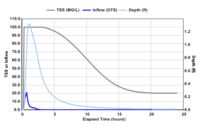
Figure 4-3 Outflow hydrograph for example conduit

Table of Contents