2.1 Introduction

Storm water runoff from urbanized areas can contain significant concentrations of harmful pollutants that can contribute to adverse water quality impacts in receiving streams. Effects can include such things as beach closures, shellfish bed closures, limits on fishing and limits on recreational contact in waters that receive storm water discharges.

Contaminants enter storm water from a variety of sources in the urban landscape. The major sources include residential and commercial areas, industrial activities, construction, streets and parking lots, and atmospheric deposition. Contaminants commonly found in storm water runoff and their likely sources are summarized in Table 2-1. Table 2-2 lists typical pollutant loadings from different urban land uses.

Table 2‑1 Sources of contaminants in urban storm water runoff (US EPA, 1999)

Contaminant	Contaminant Sources
Sediment and Floatables	Streets, lawns, driveways, roads, construction activities, atmospheric deposition, drainage channel erosion
Pesticides and Herbicides	Residential lawns and gardens, roadsides, utility right-of-ways, commercial and industrial landscaped areas, soil wash-off
Organic Materials	Residential lawns and gardens, commercial landscaping, animal wastes
Metals	Automobiles, bridges, atmospheric deposition, industrial areas, soil erosion, corroding metal surfaces, combustion processes
Oil and Grease / Hydrocarbons	Roads, driveways, parking lots, vehicle maintenance areas, gas stations, illicit dumping to storm drains
Bacteria and Viruses	Lawns, roads, leaky sanitary sewer lines, sanitary sewer cross-connections, animal waste, septic systems
Nitrogen and Phosphorus	Lawn fertilizers, atmospheric deposition, automobile exhaust, soil erosion, animal waste, detergents

Table 2‑2 Typical pollutant loadings from runoff by urban land use (lbs/acre-yr)

Land Use	TSS	TP	TKN	NH₃-N	NO₂+NO₃-N	BOD	COD	Pb	Zn	Cu
Commercial	1000	1.5	6.7	1.9	3.1	62	420	2.7	2.1	0.4
Parking Lot	400	0.7	5.1	2	2.9	47	270	0.8	0.8	0.04
HDR	420	1	4.2	0.8	2	27	170	0.8	0.7	0.03
MDR	190	0.5	2.5	0.5	1.4	13	72	0.2	0.2	0.14
LDR	10	0.04	0.03	0.02	0.1	NA	NA	0.01	0.04	0.01
Freeway	880	0.9	7.9	1.5	4.2	NA	NA	4.5	2.1	0.37
Industrial	860	1.3	3.8	0.2	1.3	NA	NA	2.4	7.3	0.5
Park	3	0.03	1.5	NA	0.3	NA	2	0	NA	NA
Construction	6000	80	NA	NA	NA	NA	NA	NA	NA	NA

HDR: High Density Residential, MDR: Medium Density Residential, LDR: Low Density Residential

NA: Not available; insufficient data to characterize loadings

Source: Burton and Pitt (2002).

The most comprehensive study of urban runoff was conducted by US EPA between 1978 and 1983 as part of the National Urban Runoff Program (NURP) (US EPA, 1983). Sampling was conducted for 28 NURP projects which included 81 specific sites and more than 2,300 separate storm events. NURP also examined coliform bacteria and priority pollutants at a subset of sites. Median event mean concentrations (EMCs) for ten general NURP pollutants for various urban land use categories are presented in Table 2-3. Fecal coliform is the most widely used indicator for the presence of harmful pathogens. Its concentration measured in separate urban storm sewers has varied widely, ranging between 400-50,000 MPN/100 ml.

Table 2‑3 Median event mean concentrations for urban land uses

Pollutant	Units	Residential		Mixed		Commercial		Open/Non-Urban
		Median	COV	Median	COV	Median	COV	Median	COV
BOD	mg/L	10	0.41	7.8	0.52	9.3	0.31	-	-
COD	mg/L	73	0.55	65	0.58	57	0.39	40	0.78
TSS	mg/L	101	0.96	67	1.14	69	0.85	70	2.92
Total Lead	μg/L	144	0.75	114	1.35	104	0.68	30	1.52
Total Copper	μg/L	33	0.99	27	1.32	29	0.81	-	-
Total Zinc	μg/L	135	0.84	154	0.78	226	1.07	195	0.66
Total Kjeldahl Nitrogen	μg/L	1900	0.73	1288	0.50	1179	0.43	965	1.00
Nitrate + Nitrite	μg/L	736	0.83	558	0.67	572	0.48	543	0.91
Total Phosphorus	μg/L	383	0.69	263	0.75	201	0.67	121	1.66
Soluble Phosphorus	μg/L	143	0.46	56	0.75	80	0.71	26	2.11

COV: Coefficient of variation

Source: Nationwide Urban Runoff Program (US EPA 1983)

2.2 Pollutant Sources

SWMM can consider several different types of pollutant sources that contribute to water quality impairment in urban catchments.

Precipitation

The chemical composition associated with precipitation, also known as wet deposition, represents a direct contribution to the water quality associated with surface runoff. Precipitation quality has been extensively monitored and varies widely by location and time of year. It can contain significant amounts of nitrates, nitrites, sulfates, sulfides, and even mercury (US EPA, 1997). SWMM accounts for this source by allowing the user to specify a constant concentration of constituents in precipitation.

Surface Runoff

For most SWMM applications, surface runoff will be the primary origin of water quality constituents. Several mechanisms contribute to stormwater runoff quality, most notably buildup and washoff. In an impervious urban area, it is usually assumed that a supply of constituents builds up on the land surface during dry weather preceding a storm. Such a buildup may or may not be a function of time and factors such as traffic flow, dry fallout (dry deposition) and street sweeping (James and Boregowda, 1985). When a storm event occurs, some fraction of this material is then washed off into the drainage system. The physics of the washoff may involve rainfall energy, as in some erosion calculations, or may be a function of bottom shear stress in the flow as in sediment transport theory. Most often, however, washoff is treated by an empirical equation with slight physical justification. Methods for predicting urban runoff quality constituents are reviewed extensively by Huber (1985, 1986), Donigian and Huber (1991), Novotny and Olem (1994), and Donigian et al. (1995).

Erosion of "solids" from soil covering the undeveloped, pervious areas of a subcatchment is another likely source of constituents. This can be modeled as a separate land use category with an unlimited amount of buildup with its own dedicated washoff equation.

Dry Weather Flow

Dry weather flow (DWF) is the continuous discharge of sanitary or industrial wastewater directly into the conveyance portion of a SWMM model, typically at junction nodes of a sanitary sewer network (refer to Figure 1-2). Thus it is only relevant when modeling sanitary or combined sewer systems. DWF usually follows some repeating pattern on both a diurnal, daily, and monthly basis. SWMM allows one to define how both the flow rate and concentration of water quality constituents vary periodically with time at any specific node of the drainage network. More information on dry weather source concentrations and flow patterns is presented in section 2.5.

Groundwater Flow

SWMM models that contain a groundwater component can generate lateral groundwater flow out of the saturated zone of a subcatchment's sub-surface area into a node of the conveyance network (see Chapter 5 of Volume I). This process is usually reserved for modeling recession curves and base flows in the open channel portions of the drainage network. One can assign constant concentrations to this flow for each water quality constituent being modeled. No attempt is made to track the transport and transformation of constituents that infiltrate from the surface into the unsaturated groundwater zone and then percolate into the saturated zone from which they enter the drainage network. Likewise, the migration of constituents from other parts of the groundwater aquifer is also ignored. Although there are many unsaturated/saturated 2-D/3-D groundwater models available that can consider such phenomena (Bear and Cheng, 2010), their complexity precludes their use within a general purpose urban drainage model like SWMM.

Inflow/Infiltration (I/I)

SWMM's hydrology module is also capable of estimating rainfall dependent inflow and infiltration (RDII) in to sewers. These are flows due to "inflow" from direct connections of downspouts, sump pumps, foundation drains, etc. as well as "infiltration" of subsurface water through cracked pipes, leaky joints, and poor manhole connections. As with groundwater, one can assign a constant concentration to water quality constituents associated with RDII flows. The same limitations of using a constant concentration here as for groundwater flow applies. Because RDII analysis is most commonly used to assess the hydraulic capacity of sanitary sewer systems, such analyses rarely consider water quality.

External Inflows

SWMM's hydraulic module (see Volume II) allows one to introduce externally imposed flows at any point in the conveyance network of channels, pipes and sewers. These flows can have water quality constituents associated with them. The constituent concentration of the inflow at some point in time is given by the following expression:

Concentration at time t = (baseline value) × (baseline pattern factor) + (scale factor) × (time series value at time t)

The baseline value is some constant, the baseline pattern is either a repeating hourly, daily, or monthly multiplier factor applied to the baseline value, the time series value is a time varying value, and the scale factor is a constant multiplier applied to each time series value. All values and factors are user-supplied. Time series values can be specified at unequal intervals of time. Interpolation is used to obtain values at intermediate times.

The expression for constituent concentration is multiplied by the flow rate associated with the external inflow to arrive at an external mass inflow rate (in units of mass per time). Instead of specifying the concentration of the external inflow one can instead use the above expression to model a time-varying mass loading of a constituent. In this case it is not necessary to provide an external flow rate to introduce a pollutant into the drainage system.

To summarize, SWMM can model water quality constituents entering a drainage system from direct precipitation, from surface runoff, from lateral groundwater flow, from rainfall dependent inflow/infiltration, from dry weather base flow or sanitary sewage flow, and from user-supplied external time series flows.

2.3 Pollutant and Land Use Objects

2.3.1 Pollutant Object

SWMM represents a water quality constituent through a Pollutant object. Any number of pollutants may be defined in a SWMM model and be included in a simulation provided that:

they can be expressed as a concentration of either mass or number (for biological organisms) per volume of water,
their masses are additive, meaning that the concentration of two equal volumes of water mixed together is the sum of the individual concentrations.

Note that these conditions would preclude naming pH as a constituent since it is expressed as the logarithm of a concentration and the pH of a mixture also depends in a nonlinear fashion on the alkalinity in the volumes being mixed. Other constituents not meeting these criteria include conductivity, turbidity, and color.

The following user-supplied properties are associated with each pollutant object:

Units – either mg/L or μg/L for chemical constituents or counts/L for biological constituents.
Rain Concentration – the concentration of the constituent in direct precipitation.
Groundwater Concentration – the concentration of the constituent in the saturated groundwater zone associated with all subcatchments in which groundwater is modeled.
Inflow/Infiltration Concentration – the concentration of the constituent in any flow that enters the conveyance system (which would typically be a sanitary sewer system) due to rainfall dependent inflow/infiltration.
Dry Weather Flow Concentration – the average concentration of the constituent in any dry weather flow (typically sanitary sewage flow) introduced externally into the conveyance system.
Decay Coefficient – a first order reaction coefficient (in units of 1/days) used to compute the rate at which the constituent decays due to reaction or other processes once it enters the conveyance portion of a SWMM model.
Snow Only Flag – a flag used to indicate if the constituent only builds up on the land surface when snow is present (such as might be the case for chlorides associated with street de-icing operations).
Co-Pollutant – the name of another pollutant whose concentration adds to the concentration of the current pollutant.
Co-Fraction – the fraction of the co-pollutant that adds to the concentration of the current pollutant.

Co-pollutants are useful for representing constituents that can appear in either dissolved or solid forms (e.g., BOD, metals, phosphorus) and may be adsorbed onto other constituents (e.g., pesticides onto "solids") and thus be generated as a portion or fraction of such other constituents. This co-fraction, also known as a potency factor, is commonly used in agricultural and sediment runoff models, such as HSPF (Bicknell et al., 1997), to relate concentrations of particulate forms of specific constituents (such as phosphorous, BOD, heavy metals, and organic nitrogen) to suspended solids concentrations. The co-fractions (or potency factor) must honor the units used for the two constituents being related. Thus a co-fraction can be greater than 1. In SWMM co-pollutants only apply to buildup/washoff processes – not to the user-specified concentrations in rainwater, groundwater, sewer inflow/infiltration (I/I), and dry weather flow.

Table 2-4 lists potency factors for suspended solids derived from wet weather sampling for different constituents and land uses in the Detroit Metropolitan area. Table 2-5 does the same for the Patuxent River basin in Maryland. The differences in factors for the same constituent at the two locations underscore how site-specific these factors can be.

2.3.2 Land Use Object

Because buildup data clearly show that different rates apply to different land uses, SWMM allows one to define different buildup and washoff functions for each combination of pollutant and land use. SWMM's Land Use object is used to identify a particular type of land use and to store the buildup (and washoff) functions for each SWMM Pollutant.

Land Uses are categories of development activities or land surface characteristics assigned to subcatchments. Examples of land use activities are residential, commercial, industrial, and undeveloped. Land surface characteristics might include rooftops, lawns, paved roads, undisturbed soils, etc. Land uses are used solely to account for spatial variation in pollutant buildup and washoff rates within subcatchments.

Table 2‑4 Potency factors for the Detroit metropolitan area (mg/gram) Source: Roesner (1982).

Constituent	Residential	Commercial/Industrial	Roads	Rural
BOD5	34	45	10	18
Fecal Coliforms^a	87,000	37,000	200,000	300,000
NH₄	0.8	2.4	0.35	0.45
NO₂ + NO₃	1.7	6.4	0.07	3.5
Total Organic N	4.3	4.1	1.22	7.0
Total P	1.9	1.7	0.26	1.5
PO₄	0.24	0.47	0.20	2.4
Oil & Grease	25	80	100	13
Lead	1.8	1.4	0.41	0.21

^a (organisms/100ml) / (gram/L TSS)

Table 2‑5 Potency factors for the Patuxent River Basin (mg/gram) Source: Aqua Terra (1994).

Land Use	NO₃	NH₄	PO₄	BOD
Low Density Residential	1.5	0.4	1.1	90
Medium/High Density Residential	6.0	2.0	1.6	180
Commercial/Industrial	10.0	3.2	2.7	270
Forest and Wetland	0.1-0.18	0.011-0.018	0.04-0.07	11-17
Pasture	3.6	0.4	0.27	60
Idle Agricultural Land	2.0	0.2	0.16	30

The SWMM user has many options for defining land uses and assigning them to subcatchment areas. One approach is to assign a mix of land uses for each subcatchment, which results in all land uses within the subcatchment having the same pervious and impervious characteristics. Another approach is to create subcatchments that have a single land use classification along with a distinct set of pervious and impervious characteristics that reflects the classification. If surface buildup and washoff is not being modeled, such as when pollutant inflows come only from wet deposition, dry weather sanitary flows, and external time series flows, then there is no need to add land uses into a project.

2.4 Wet Deposition

There is considerable public awareness of the fact that precipitation is by no means "pure" and does not have characteristics of distilled water. Low pH (acid rain) is the best known parameter but many substances can also be found in precipitation, including organics, solids, nutrients, metals and pesticides (Novotny and Olem, 1994). Atmospheric deposition is an important loading factor in coastal waters (NRC, 2000). Compared to surface sources, rainfall is probably an important contributor mainly of some nutrients in urban runoff, although it may contribute substantially to other constituents as well. In particular, Kluesener and Lee (1974) found ammonia levels in rainfall higher than in runoff in a residential catchment in Madison, Wisconsin; rainfall nitrate accounted for 20 to 90 percent of the nitrate in stormwater runoff to Lake Wingra. Mattraw and Sherwood (1977) report similar findings for nitrate and total nitrogen for a residential area near Fort Lauderdale, Florida. Data from the latter study are presented in Table 2-6 in which rainfall may be seen to be an important contributor to all nitrogen forms, plus COD, although the instance of a higher COD value in rainfall than in runoff is probably anomalous.

In addition to the two references first cited, Weibel et al. (1964, 1966) report concentrations of constituents in Cincinnati rainfall (Table 2-6), and a summary is also given by Manning et al. (1977). Other data on rainfall chemistry and loadings are given by Uttormark et al. (1974), Betson (1978), Hendry and Brezonik (1980), Novotny and Kincaid (1981), Randall et al. (1981), Mills et al., (1985), and Novotny and Olem (1994). A comprehensive summary is presented by Brezonik (1975) from which it may be seen in Table 2-6 that there is a wide range of concentrations observed in rainfall. Again, the most important parameters relative to urban runoff are probably the various nitrogen forms.

The previous cited literature reflects relevant but older information regarding precipitation chemistry. A very useful web site is http://nadp.sws.uiuc.edu/, for the National Atmospheric Deposition Program (NADP). Data may be downloaded from this site for hundreds of monitoring locations across the U.S., permitting good estimates of regional precipitation concentrations. Annual, seasonal, and time series data and plots may be downloaded for wet and dry deposition of parameters such as pH, nitrogen species, calcium, chloride, and whatever else is measured at a site. A bonus for some sites is daily precipitation data. Dry deposition values might be included with buildup on the land surface, although other buildup factors, such as wind erosion, traffic, etc. make it very difficult to separate causative factors (James and Boregowda, 1985).

Table 2‑6 Representative concentrations of constituents in rainfall

Parameter	Ft. Lauderdale^a	Cincinnati^b	Lodi, NJ^c	"Typical Range"^d
Acidity
pH				3-6
Organics
BOD5, mg/L	4-22	16		1-13
COD, mg/L	1-3			9-16
TOC, mg/L	0-2			Few
Inorg. C, mg/L
Color
PCU	5-10
Solids
Total Solids, mg/L	18-24	13
Suspended Solids, mg/L	2-10
Turbidity, JTU	4-7
Nutrients
Org. N, mg/L	0.09-0.15	0.58		0.05-1.0
NH₃-N, mg/L	0.01-0.04	1.27^e		0.05-1.0
NO₂-N, mg/L	0.00-0.01	0.08		0.2-1.5
NO₃-N, mg/L	0.12-0.73			0.0-0.05
Total N, mg/L	0.29-0.84			0.02-0.15
Orthophosphorus, mg/L	0.01-0.03
Total P, mg/L	0.01-0.05
Pesticides
μg/L		3-600		Few
Heavy metals
Lead, μg/L			45	30-70
Nickel, μg/L			3
Copper, μg/L			6
Zinc, μg/L			44

^aRange for three storms (Mattraw and Sherwood, 1977)
^bAverage of 35 storms (Weibel et al., 1966)
^cWilbur and Hunter (1980)
^dBrezonik (1975)
^eSum of NH₃-N, NO₂-N, NO₃-N

Constituent concentrations in precipitation are associated with a SWMM Pollutant object. All surface runoff, including snowmelt, is assumed to have at least this concentration, and the precipitation load is calculated by multiplying this concentration by the runoff rate and adding to the load already generated by other mechanisms. It may be inappropriate to add a precipitation load to loads generated by a calibration of buildup-washoff or rating curve parameters against measured runoff concentrations, since the latter already reflect the sum of all contributions, land surface and otherwise. But precipitation loads might well be included if starting with buildup-washoff data from other sources. They also provide another simple means for imposing a constant concentration on any subcatchment constituent.

2.5 Dry Weather Flow

For most of this discussion, "dry-weather flow" (DWF), equivalent to base flow in a natural stream, is derived from sanitary sewage or industrial flows entering the drainage system – usually a combined sewer. Since SWMM can also be used to simulate sanitary sewers and systems with cross connections, DWF might also be applied to simulations of those systems. The estimation of DWF quantity and quality in a sewer system can be broken into two parts: 1) estimates of average quantities, and 2) estimates of time patterns to apply to these averages. The discussion that follows addresses each of these aspects.

2.5.1 Average Dry-Weather Flow Estimates

Like almost all SWMM input parameters, DWF hydrographs and pollutographs are best determined through monitoring. Monitoring of inflows to a municipal wastewater treatment plant (WWTP) is routinely performed, at least for flow. This end-of-pipe discharge may then be apportioned back through the sewer system on the basis of population through census tract data, as a first approximation. Similarly, population estimates are often used as the basis to determine DWF, on a per capita basis. These per capita estimates vary considerably. For instance, ASCE-WPCF (1969) report per capita data for 34 cities, as summarized in Table 2-7. Data in this table are from the 1960s and reflect sewage discharges at that time; modern cities tend to have less per capita water use due to low-volume plumbing fixtures, etc. Water use itself is another surrogate for DWF measurements, especially winter values that reflect indoor use only (no irrigation, car washing, etc.).

Many other sources contribute to average DWF, including commercial establishments, hospitals, municipal and institutional buildings, apartment buildings, etc., none of which are easily represented on a per capita basis. Environmental engineering texts, such as Metcalf & Eddy, Inc. (2003) provide tables with data from such locations. Industries can generate large quantities of DWF and must be evaluated individually. Another alternative for DWF estimates is on a per area basis, but such design curves (gallons per acre per day vs. acres) are highly site-specific (ASCE-WPCF, 1969).

Table 2‑7 Average daily dry weather flow in 29 cities Source: ASCE-WPCF (1969)

#	City	Avg. Sewage Flow, gpd/cap	#	City	Avg. Sewage Flow, gpd/cap
1	Baltimore, MD	100	19	Los Angeles 2, CA	70
2	Berkeley, CA	60	20	Greater Peoria, IL	75
3	Boston, MA	140	21	Milwaukee, WI	125
4	Cleveland, OH	100	22	Memphis, TN	100
5	Cranston, RI	119	23	Orlando, FL	70
6	Des Moines, IA	100	24	Painesville, OH	125
7	Grand Rapids, MI	190	25	Rapid City, SD	121
8	Greenville County, SC	150	26	Santa Monica, CA	92
9	Hagerstown, MD	100	27	St. Joseph, MO	125
10	Jefferson County, AL	100	28	Washington, DC	100
11	Johnson County-1, KS	60	29	Wyoming, MI	82
12	Johnson County 2, KS	60
13	Kansas City, MO	60
14	Lancaster County, NB	92
15	Las Vegas, NV	209
16	Lincoln, NB	60
17	Little Rock, AR	50
18	Los Angeles, CA	85

Summary Statistics:

Average: 101
CV*: 0.38
Maximum: 209
Minimum: 50
Median: 100

*CV = coefficient of variation = standard deviation/average

Table 2‑8 Quality properties of untreated domestic wastewater Source: Metcalf and Eddy, Inc. (2003)

Contaminant	Unit	Weak	Medium	Strong
Solids, total	mg/L	390	720	1230
Solids, total dissolved (TDS)	mg/L	270	500	860
Fixed	mg/L	160	300	520
Volatile	mg/L	110	200	340
Solids, suspended, total (TSS)	mg/L	120	210	400
Fixed	mg/L	25	50	85
Volatile	mg/L	95	160	315
Solids, settleable	mg/L	5	10	20
Biochemical oxygen demand, 5-day (BOD5)	mg/L	110	190	350
Total organic carbon (TOC)	mg/L	80	140	260
Chemical oxygen demand (COD)	mg/L	250	430	800
Nitrogen, total as N (TN)	mg/L	20	40	70
Organic	mg/L	8	15	25
Free ammonia (NH3)	mg/L	12	25	45
Nitrite (NO2)	mg/L	0	0	0
Nitrate (NO3)	mg/L	0	0	0
Phosphorus, total as P (TP)	mg/L	4	7	12
Organic	mg/L	1	2	4
Inorganic	mg/L	3	5	10
Chlorides	mg/L	30	50	90
Sulfate	mg/L	20	30	50
Oil and Grease	mg/L	50	90	100
Volatile organic compounds (VOCs)	mg/L	<100	100-400	>400
Total coliform	#/100 mL	10⁶-10⁸	10⁷-10⁹	10⁷-10¹⁰
Fecal coliform	#/100 mL	10³-10⁵	10⁴-10⁶	10⁵-10⁸

"Weak" is based on an approximate wastewater flow rate of 200 gpd/day (750 L/capita-day, "medium" of 120 gpd/day (460 L/capita-day), and "strong" of 60 gpd/day (240 L/capita-day).

Domestic wastewater quality is variable, but well documented. Typical values are shown in Table 2-8 (Metcalf and Eddy, Inc., 2003). Estimates are also available on a per capita basis (unit loads) of the type shown in Table 2-9 and expanded upon in texts such as Metcalf and Eddy, Inc. (2003). Commercial, industrial, and institutional quality is typically stronger (higher concentrations) than domestic wastewater and should be evaluated individually. Guidelines may be found in several sources, such as Tchobanoglous and Burton (1991) and Metcalf and Eddy Inc. (2003). Earlier SWMM documentation provides additional literature reviews on these topics (Metcalf and Eddy et al., 1971a; Huber and Dickinson, 1988).

Table 2‑9 Unit quality loads for domestic sewage, including effects of garbage grinders Source: Haseltine (1950); Metcalf and Eddy et al. (1971a).

Constituent	Sewage (lb/capita-day)	Ground Garbage (lb/capita-day)
Total solids	0.55	0.15
Total volatile solids	0.32	0.13
Suspended matter	0.20	0.10
BOD5	0.17	0.08
Fats and greases	0.05	0.03
Total nitrogen	0.04	0.002

2.5.2 Temporal Variations in Dry-Weather Flow

Dry-weather flow quantity and quality varies seasonally, weekly, and daily. SWMM provides monthly (one multiplier for each month of year), daily (one multiplier for each day of week), hourly (one multiplier for each hour of day), and weekend (one multiplier for each hour of weekend days) adjustment factors to be applied to average DWF quantities. Typical sinusoidal variations are shown in texts such as Metcalf and Eddy Inc. (2003) and in ASCE and WPCF (1969), but these variations are best obtained by examination of WWTP inflow hydrographs. Variations in daily water use (surrogate for wastewater discharge) reported for nine homes monitored in November 1964 by Tucker (1967) are shown in Table 2-10. Typical hourly variations in domestic wastewater flow and strength given by Metcalf and Eddy, Inc. (2003) are shown in Figure 2-1 and Table 2-11.

Table 2‑10 Autumn water use for six homes near Wheaton, MD Source: Tucker (1967).

Week	Sun	Mon	Tues	Wed	Thurs	Fri	Sat	Average
Six home use, gal (10/18/64)	1722	2137	1941	1938	1706	1777	1762	1855
Ratio to avg.	0.928	1.152	1.047	1.045	0.920	0.958	0.950

Six home use, gal (11/1/64)	1774	1569	1966	1714	1663	1861	1784	1762
Ratio to avg.	1.007	0.891	1.116	0.973	0.944	1.056	1.013

Average ratios	0.968	1.021	1.081	1.009	0.932	1.007	0.981	1.000

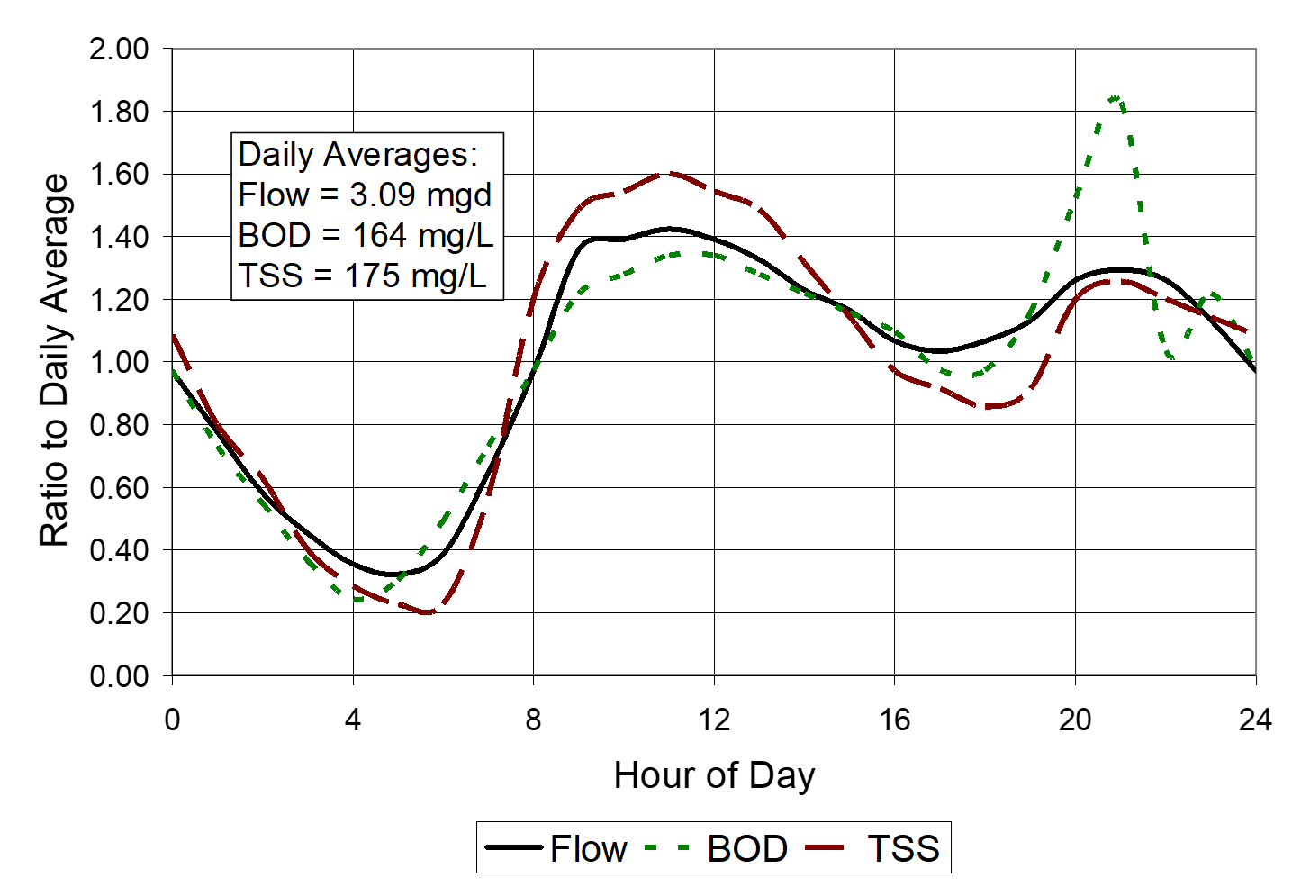
Figure 2‑1 Hourly domestic sewage time patterns

(Based on data from Metcalf and Eddy, Inc.(2003). Ratios are based on indicated daily averages.)

Table 2‑11 Typical hourly DWF correction factors Source: Metcalf and Eddy, Inc. (2003).

Hour	Flow	BOD	TSS	Hour	Flow	BOD	TSS
1	0.78	0.73	0.80	13	1.33	1.28	1.49
2	0.58	0.55	0.63	14	1.23	1.22	1.31
3	0.45	0.37	0.40	15	1.16	1.16	1.14
4	0.36	0.24	0.29	16	1.07	1.10	0.97
5	0.32	0.30	0.23	17	1.04	0.97	0.91
6	0.39	0.49	0.23	18	1.07	0.97	0.86
7	0.65	0.73	0.57	19	1.13	1.16	0.91
8	0.97	0.97	1.20	20	1.26	1.52	1.20
9	1.36	1.22	1.49	21	1.29	1.83	1.26
10	1.39	1.28	1.54	22	1.26	1.04	1.20
11	1.42	1.34	1.60	23	1.13	1.22	1.14
Noon	1.39	1.34	1.54	Midnight	0.97	0.97	1.09
				Average	1.00	1.00	1.00

2.6 Simulating Runoff Quality

Simulation of urban runoff quality is a very inexact science if it can even be called such. Very large uncertainties arise both in the representation of the physical, chemical and biological processes and in the acquisition of data and parameters for model algorithms. For instance, subsequent sections will discuss the concept of "buildup" of pollutants on land surfaces and "washoff" during storm events. The true mechanisms of buildup involve factors such as wind, traffic, atmospheric fallout, land surface activities, erosion, street cleaning and other imponderables. Although efforts have been made to include such factors in physically-based equations (James and Boregowda, 1985), it is unrealistic to assume that they can be represented with enough accuracy to determine a priori the amount of pollutants on the surface at the beginning of the storm. Equally naive is the idea that empirical washoff equations truly represent the complex hydrodynamic (and chemical and biological) processes that occur while overland flow moves in random patterns over the land surface. The many difficulties of simulation of urban runoff quality are discussed by Huber (1985, 1986).

Such uncertainties can be dealt with in two ways. The first option is to collect enough calibration and verification data to be able to calibrate the model equations used for quality simulation. Given sufficient data, the equations used in SWMM can usually be manipulated to reproduce measured concentrations and loads. This is essentially the option discussed at length in the following sections. The second option is to abandon the notion of detailed quality simulation altogether and either use a constant concentration (event mean concentration or EMC) applied to quantity predictions (i.e., obtain storm loads by multiplying predicted volumes by an assumed concentration) (Johansen et al., 1984) or use a statistical method (Hydroscience, 1979; Driscoll and Assoc., 1981; US EPA, 1983b; DiToro, 1984; Adams and Papa, 2000). EMC values may be entered directly into SWMM 5. Statistical methods are based in part upon strong evidence that storm event mean concentrations are lognormally distributed (Driscoll, 1986). The statistical methods recognize the frustrations of physically-based modeling and move directly to a stochastic result (e.g., a frequency distribution of EMCs), but they are even more dependent on available data than methods such as those found in SWMM. That is, statistical parameters such as mean, median and variance must be available from other studies in order to use the statistical methods. Furthermore, it is harder to study the effect of controls and catchment modifications using statistical methods.

Table 4-12 on p. 4-77.The main point is that there are alternatives to the buildup-washoff approach available in SWMM; the latter can involve extensive effort at parameter estimation and model calibration to produce quality predictions that may vary greatly from an unknown "reality." But SWMM also offers simpler options, including the constant concentration or EMC approach. Before delving into the arcane methods incorporated in SWMM and other urban runoff quality simulation models, the user should try to determine whether or not the effort will be worth it in view of the uncertainties of the process and whether or not simpler alternative methods might suffice. The discussions that follow provide a comprehensive view of the options available in SWMM, which are more than in almost any other comparable model, but the extent of the discussion should not be interpreted as a guarantee of success in applying the methods.

Although the conceptualization of the quality processes is not difficult, the reliability and credibility of quality parameter simulation is very challenging to establish. In fact, quality predictions by SWMM or almost any other surface runoff model are mostly hypothetical unless local data for the catchment being simulated are available to use for calibration and validation. If such data are lacking, results may still be used to compare relative effects of changes, but parameter magnitudes (i.e., actual values of predicted concentrations) will forever be in doubt. This is in marked contrast to quantity prediction for which reasonable estimates of hydrographs may be made in advance of calibration.

Moreover, there is disagreement in the literature as to what are the important and appropriate physical and chemical mechanisms that should be included in a model to generate surface runoff quality. The objective in SWMM has been to provide flexibility in mechanisms and the opportunity for calibration. But this places a considerable burden on the user to obtain adequate data for model usage and to be familiar with quality mechanisms that may apply to the catchment being studied. This burden is all too often ignored, leading ultimately to model results being discredited.

In the end then, there is no substitute for local data (rain, flow, and concentration measurements) with which to calibrate and verify the quality predictions. Without such data, little reliability can be placed in the predicted magnitudes of quality parameters.

Early quality modeling efforts with SWMM emphasized generation of detailed pollutographs, in which concentrations versus time were generated for short time increments during a storm event (e.g., Metcalf and Eddy et al., 1971b). Depending upon the application, such detail may be entirely unnecessary because the receiving waters cannot respond to such rapid changes in concentration or loads. Instead, only the total storm event load is necessary for most studies of receiving water quality. Time scales for the response of various receiving waters are presented in Table 2-12 (Driscoll, 1979; Hydroscience, 1979). Concentration transients occurring within a storm event are unlikely to affect any common quality parameter within the receiving water, with the possible exception of bacteria. Detailed temporal concentration variations within a storm event are needed primarily when they will affect control alternatives. For example, a storage device may need to trap the "first flush" of pollutants, if one exists.

Table 2‑12 Required temporal detail for receiving water analysis Source: Driscoll (1979) and Hydroscience (1979).

Type of Receiving Water	Key Constituents	Response Time
Lakes, Bays	Nutrients	Weeks - Years
Estuaries	Nutrients, DO	Days - Weeks
Large Rivers	DO, Nitrogen	Days
Streams	DO, Nitrogen	Hours - Days
	Bacteria	Hours
Ponds	DO, Nutrients	Hours - Weeks
Beaches	Bacteria	Hours

The significant point is that calibration and verification ordinarily need only be performed on total storm event loads, or on event mean concentrations. This is a much easier task than trying to match detailed concentration transients within a storm event.

Table of Contents