Models keep their physics. Connections share a meaning.
An output from one model becomes an input to another. The connection identifies the quantity, units, geometry and time; an adapted output performs declared transformations where needed. A workflow coordinates the models’ lifecycle and execution. HydroCouple builds on concepts from the OGC OpenMI 2.0 standard and extends them with spatial data, efficient array exchange and optional capabilities.
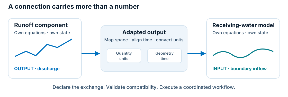
Describe
Expose identity, configuration, inputs, outputs, state and supported capabilities.
Exchange
Move values with their units, dimensions, spatial references and temporal semantics.
Coordinate
Initialize, validate, prepare, update and finish through a common lifecycle.
The interface standard defines the contract. The SDK provides implementations and workflows; models provide their own numerical methods.
Carry sensitivities through the whole cascade
A Jacobian collects derivatives of a vector of outputs with respect to a vector of inputs. A gradient describes how one scalar objective changes with its variables. HydroCouple exposes Jacobian products, so components can propagate sensitivities without assembling or storing a full Jacobian.
- Jacobian
- Local linear response of all selected outputs to the selected inputs, parameters and prior state.J = ∂y / ∂x
- JVP · forward mode
- A Jacobian–vector product sends an input tangent perturbation forward to an output tangent.δy = J δx
- VJP · reverse mode
- A vector–Jacobian product sends an objective cotangent backward. In column-vector notation:∇xL = Jᵀ ∇yL
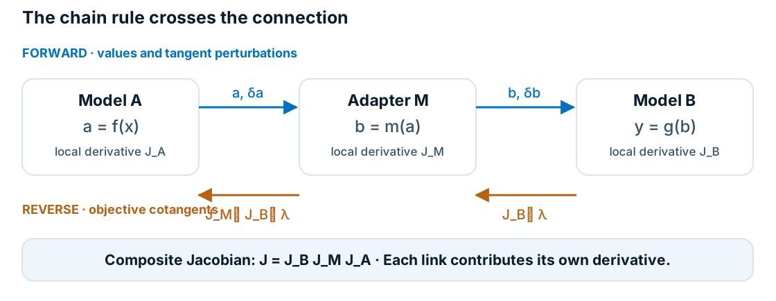
The standard specifies the derivative contract, not the differentiation method. Automatic differentiation (AD) applies the chain rule to implemented numerical operations to obtain derivatives. A component can use AD or supply analytical derivatives or a hand-written adjoint through the same JVP/VJP interfaces. Every component and adapter on the requested path must supply valid derivatives. Read the contracts →
See uncertainty and sensitivities change together
A toy cascade has two inputs and two outputs. Change an adapter’s mapping gain, input standard deviation or correlation. The composite Jacobian maps input covariance to output covariance.
Enable JavaScript to explore the example. Its calculations use J = BMA and Σy = JΣxJᵀ; all quantities are dimensionless.
Composite Jacobian J
| Input 1 | Input 2 | |
|---|---|---|
| Output 1 | ||
| Output 2 |
JVP: an input tangent (0.01, 0) gives .
VJP: for objective L = output 1, the input gradient is .
Equations and assumptions
A = [[1, 0.2], [0.1, 0.8]], M = diag(gain, 1), B = [[1.2, 0.4], [0.3, 0.9]]. J = BMA. The input covariance has variances σ₁² and σ₂² and covariance ρσ₁σ₂. This is an exact linear example, not a calibrated water model. For nonlinear models, Σy ≈ JΣxJᵀ is a local first-order approximation.
Follow state through time
A time step maps previous state, inputs and parameters to new state and outputs. Both components and adapters can carry memory. Their differentiation interfaces distinguish state before from state after; checkpointing lets a workflow restore and replay earlier steps at the correct linearization point.
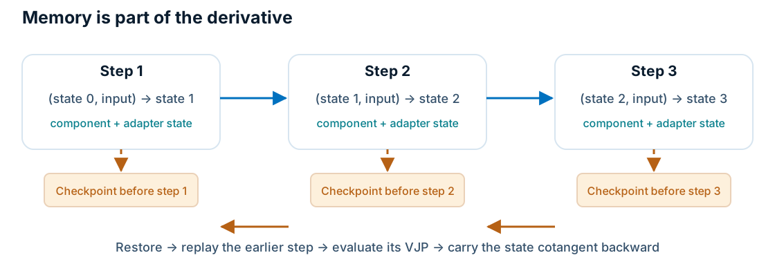
The current SDK reverse workflow supports time-stepped acyclic compositions, including differentiable, checkpointable relaxation adapters. It rejects unsupported paths rather than inventing a derivative. Feedback-loop differentiation and general multi-rate differentiation require further workflow support. Workflow scope →
From system response to system decisions
Uncertainty assessment
Trace sensitivity to forcing, parameters and initial conditions across models. Propagate correlated input covariance with a local linear approximation, then use ensembles for nonlinear behavior. Sensitivity alone is not an uncertainty estimate.
Physics-informed machine learning
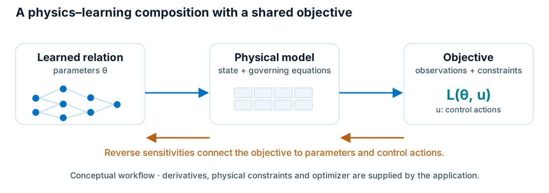
Train a learned relation inside a physical model, or use model sensitivities in an inverse problem. Physics-informed neural networks (PINNs) additionally use space/time derivatives to construct governing-equation residuals—a different derivative from a coupled model’s parameter sensitivity.
Calibration and control
Differentiate a scalar objective with respect to parameters or control actions. This can support gradient-based calibration and model predictive control (MPC). Constraints, observation quality and nonsmooth events such as valve switching still belong in the application.
Connect observations to forecasts—and decisions
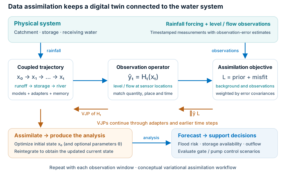
A water-system digital twin can connect a physical catchment, storage network and receiving water to a model that is continually updated from observations. Data assimilation combines these observations with a prior forecast (the background), accounting for their uncertainties, to estimate an updated state (the analysis) for the next forecast. NIST: digital twin elements · ECMWF: assimilation terminology
Observe in model space
An observation operator maps model state to the quantity, location and time of a measurement. Level and flow observations can inform unobserved storage and upstream states through their modeled connections.
Differentiate the mismatch
Four-dimensional variational data assimilation (4D-Var) adjusts initial conditions over an observation window. AD can supply the objective gradient through the model trajectory and observation operators; HydroCouple’s VJPs carry it across component boundaries.
Update, forecast, control
Reintegrate from the optimized initial state to obtain the current analysis. Start the next forecast from that state and evaluate control actions against downstream risk and available storage. Repeat as new observations arrive.
Variational assimilation minimizes a background penalty plus observation misfit, weighted by their error covariances. ECMWF: gradients and adjoints in 4D-Var
This illustrates an application the interfaces can support when all participating paths provide derivatives and replay. Assimilation, sensor quality checks, error covariances and the optimizer are application responsibilities. Ensemble Kalman filters offer another assimilation approach and do not require explicit model derivatives.
Shared data, flexible execution
Spatial and temporal meaning
Geometries, meshes, networks, rasters and layered domains describe where values apply. Time-series and time-marching interfaces describe when they apply.
Efficient array exchange
Typed buffers declare shape, strides and memory space for efficient C++, Python and accelerator exchange. Quantities declare units and how values behave when mapped or aggregated.
Parallel and distributed workflows
Cloning supports independent ensemble members. Distributed interfaces describe transports, remote components and partitioned data. Implementations choose the runtime and execution backend.
Geometry follows OGC Simple Feature Access concepts. SDK and engine I/O can use OGC GeoPackage, NetCDF or HDF5; these file formats are distinct from the runtime coupling interface.
Explore the main interface contracts
| Concern | Interface | Responsibility |
|---|---|---|
| Model execution | IModelComponent | Lifecycle, inputs, outputs, arguments, state, capabilities and diagnostics. |
| Data and adaptation | IComponentDataItem, IInput, IOutput, IAdaptedOutput | Typed data, connections and declared transformations. |
| Differentiation | IDifferentiableModelComponent, IDifferentiableAdaptedOutput | JVPs and VJPs of the most recent update or refresh. |
| Replay | ICheckpointableModelComponent, ICheckpointableAdaptedOutput | Save, restore and release state for earlier-step replay. |
| Composition | IWorkflowComponent, ICloneableModelComponent | Coordinate components and create independent component instances. |
| Distributed data | ITransport, IPartitionedComponentDataItem | Transport-neutral messaging and partitioned fields. |
Read the standard. Explore its implementations.
AI tools assisted with the writing and illustrative figure code. Terminology and capability descriptions were checked against the HydroCouple 2.0.0-alpha.2 contracts. The interactive example is dimensionless and synthetic; it reports no operational model results.