Articles

From individual practices to distributed systems: detention, treatment, active control and receiving waters

A rain garden can perform well on its own and still be part of a drainage system that performs poorly. Its outlet may meet a high downstream water level. Several facilities may release together. Holding water for treatment may leave too little capacity for the next storm. And water that infiltrates does not necessarily disappear from the watershed.

These questions have motivated the new LID Storage node implementation in Open-Source SWMM 6 (SWMM2D). The aim is to move beyond evaluating performance of localized low impact development practices and examine the system-wide implications of distributed LIDs for receiving groundwater and water bodies: flow peaks, timing, cumulative pollutant loads and the pathways connecting facilities.

Show static figure

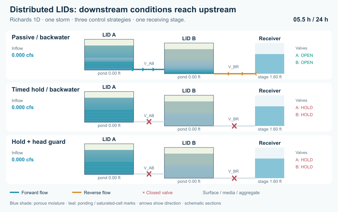
Figure 1. A simulated storm moves through two layered storage nodes. Blue arrows show forward flow; amber arrows show reversal; crosses mark closed valves. The receiving-water stage rises between hours 3 and 4, stays high until hour 7, then falls. Dots indicate direction, not tracked particles. Blue shading shows porous-cell moisture; teal marks surface ponding and saturated cells. Cross-sections are schematic and use a common head datum. Static figure.

Why the network matters

Conventional SWMM LIDs describe rainfall, infiltration and drainage within a subcatchment. SWMM can also represent treatment trains by routing runoff between dedicated subcatchments; LIDs within one subcatchment are treated in parallel. See the EPA SWMM 5.2 User's Manual.

SWMM 5 already provides LID drain controls. Version 5.1.013 (August 2018) added separate drain opening and closing water levels and a control curve that adjusts nominal drain discharge as a function of the head above the drain outlet. Each conventional LID control has one underdrain definition, one opening/closing threshold pair and one optional head-based discharge curve. This represents the combined drain response of a unit, which may contain several physical drain pipes; it does not provide separate hydraulic connections and valve settings at different elevations. These controls respond to water levels within the LID; the conventional LID underdrain calculation does not include the receiving node's downstream head. EPA release notes; EPA LID underdrain implementation.

The new work connects the layered LID directly to SWMM's existing hydraulic network and control rules. A storage-node LID can have an arbitrary number of hydraulic connections at different elevations, with separate rules for each controllable link. An orifice used to represent a valve can be closed, partially open or fully open through its setting from 0 to 1. Link flow responds to both the facility's head and the downstream head, allowing backwater to restrict drainage and, where the link permits it, reverse flow into the facility. Controls can also respond to receiving-water levels. This couples the layered water stores and treatment processes to the surrounding network.

The added flexibility comes from exposing the layered facility to SWMM's existing network links and controls. It supports coordinated operation of several outlets within one facility and across a treatment train.

For the layered facility, this supports questions such as:

• Does detention at an upstream facility reduce a downstream peak, or move it into the peak from another tributary?
• How does downstream backwater change available storage, flow direction and exposure to treatment media?
• Can a controller retain polluted runoff while preserving capacity for a second storm?
• How much pollutant is transformed, discharged, bypassed or still stored at the end of the assessment?

Research on water-quality-informed real-time control provides a motivation for asking these questions. Sharior, McDonald and Parolari studied detention-basin control using water-quality information, with outcomes dependent on rainfall conditions. Gomes Junior and colleagues examined valve-control strategies and detention/flood tradeoffs in a stormwater network. Those studies support investigating controls; they do not establish the performance of the hypothetical LID train below. Sharior et al., 2019; Gomes Junior et al., 2022.

A layered facility that remains a storage node

The implementation attaches a LID control to an ordinary storage node. Storage geometry supplies its footprint. An ordered stack supplies the surface, media and aggregate thicknesses and moisture properties. Ordinary hydraulic links supply connections to other facilities and the receiving water.

For example, a facility can have a low-level drawdown valve, an independently controlled intermediate-level outlet to a second facility, and a high-level emergency overflow. Each connection has its own elevation and hydraulic properties; the two valves can follow different schedules or opening settings. Dynamic Wave routing represents the effect of downstream head and flow reversal. Layer-relative outlet anchors follow physical stack edits; a link joining two LID nodes uses explicit endpoint offsets.

The distinction matters for water quality. In Richards mode, porous cells retain individual water and pollutant inventories, including when saturated; surface ponding is a separate mixed reservoir. The existing flow model uses retained cells plus a shared mobile-water reactor. Layer treatment can specify fixed removal, first-order decay and optional expressions. A surface bypass does not automatically receive all the treatment rules beneath it. The stack is not a sequence of independent saturated plug-flow reactors.

In the present implementation, storage-node pollutant routing uses Dynamic Wave with the Legacy quality solver. Assigning a LID does not add rainfall automatically: supply runoff through contributing subcatchments or an external inflow. Native INP and GeoPackage preserve the extension; export to legacy SWMM 5 does not preserve this behavior.

The formulation: water, head and pollutant mass

A semi-discrete Richards column inside a hydraulic node

The node now offers two flow models. Existing formulation (with backwater) retains the exponential gravity-drainage law and modified Green–Ampt surface entry used in the earlier article tests. Richards 1D resolves vertical gravity and matric-pressure gradients within MEDIA and AGGREGATE. The revised experiments below explicitly select Richards; the earlier results remain a separately labeled comparison.

Matric head ψ expresses the pressure of pore water relative to atmospheric pressure, as an equivalent water-column height. It is negative in unsaturated media: the pore matrix holds water under suction. Total hydraulic head is H = z + ψ, with upward-positive elevation z. A drier region can draw water from a wetter neighbor through this head difference, even upward against gravity. The flow direction depends on total head, while its rate also depends on how readily the partly filled pores conduct water.

The continuous one-dimensional water balance is:

∂w(ψ)/∂t = −∂q/∂z − s, with q = −K(ψ) ∂(z + ψ)/∂z

Here q is upward-positive Darcy flux and s a volumetric sink. Semi-discrete means that the column is divided into spatial control volumes while their water balances remain ordinary differential equations in time. For cells ordered from top to bottom, define Q positive downward:

Wᵢ = Gᵢ [θᵢ(ψᵢ) + S_s,ᵢ max(ψᵢ, 0)]

dWᵢ/dt = Qᵢ₋₁/₂ − Qᵢ₊₁/₂ − Eᵢ

Qᵢ₊₁/₂ = A_f K_f (Hᵢ − Hᵢ₊₁) / d_f

Gᵢ is cell geometric volume, A_f the shared face area, d_f the distance between cell centers and Eᵢ the evaporation withdrawal rate. Neighboring cells receive equal and opposite interface transfers. S_s is specific storage: when pressure becomes positive, θ stays at porosity, while elastic water storage can increase. The porous column owns all pore and elastic water; the network node owns surface ponding. Saturated pore water is not counted again in a shared mobile reactor.

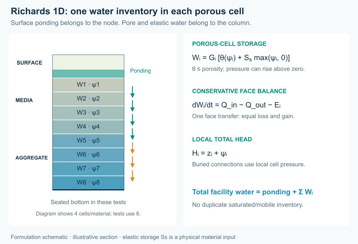
Figure 2. Water ownership in Richards mode. Every porous cell has its own water volume and pressure; surface ponding is the separate hydraulic reservoir. Numerical cells subdivide physical materials without adding new authored treatment layers. This is a formulation schematic.

How interlayer flux is calculated

Richards mode uses explicit van Genuchten retention and Mualem conductivity properties for each porous material. With m = 1 − 1/n:

Sₑ = [1 + (α |ψ|)ⁿ]⁻ᵐ for ψ < 0; Sₑ = 1 for ψ ≥ 0

θ = θᵣ + (φ − θᵣ) Sₑ

K = K_s Sₑˡ [1 − (1 − Sₑ¹/ᵐ)ᵐ]²

Residual content θᵣ, porosity φ, saturated conductivity K_s, inverse capillary-length parameter α, shape parameters n and l, and specific storage S_s must be supplied. Conductivity slope, field capacity and Green–Ampt suction from the existing model do not determine these curves. The Richards flux has no field-capacity cutoff: redistribution continues wherever conductivity and a head gradient permit it.

Within equal-size cells of one material, the face conductivity is the arithmetic mean of the two cell conductivities. Across different materials, the two half-cell resistances act in series:

Q_f = A_f (Hᵢ − Hᵢ₊₁) / [(Δzᵢ/2)/Kᵢ + (Δzᵢ₊₁/2)/Kᵢ₊₁]

Thus both sides influence interlayer flow. A positive downward Q drains the upper cell; a negative Q redistributes water upward. At the pond/media contact, the mean of saturated surface-contact conductivity and first-cell conductivity is used over half a cell thickness. Downward entry smoothly tends to zero through the last 1 micrometre of ponding; upward return remains possible. No separate Green–Ampt front is evolved in Richards mode. The spatial approach draws on the method-of-lines formulation described by Ireson et al. (2023), openRE; the implementation here has its own storage variables, boundary coupling and time integrator.

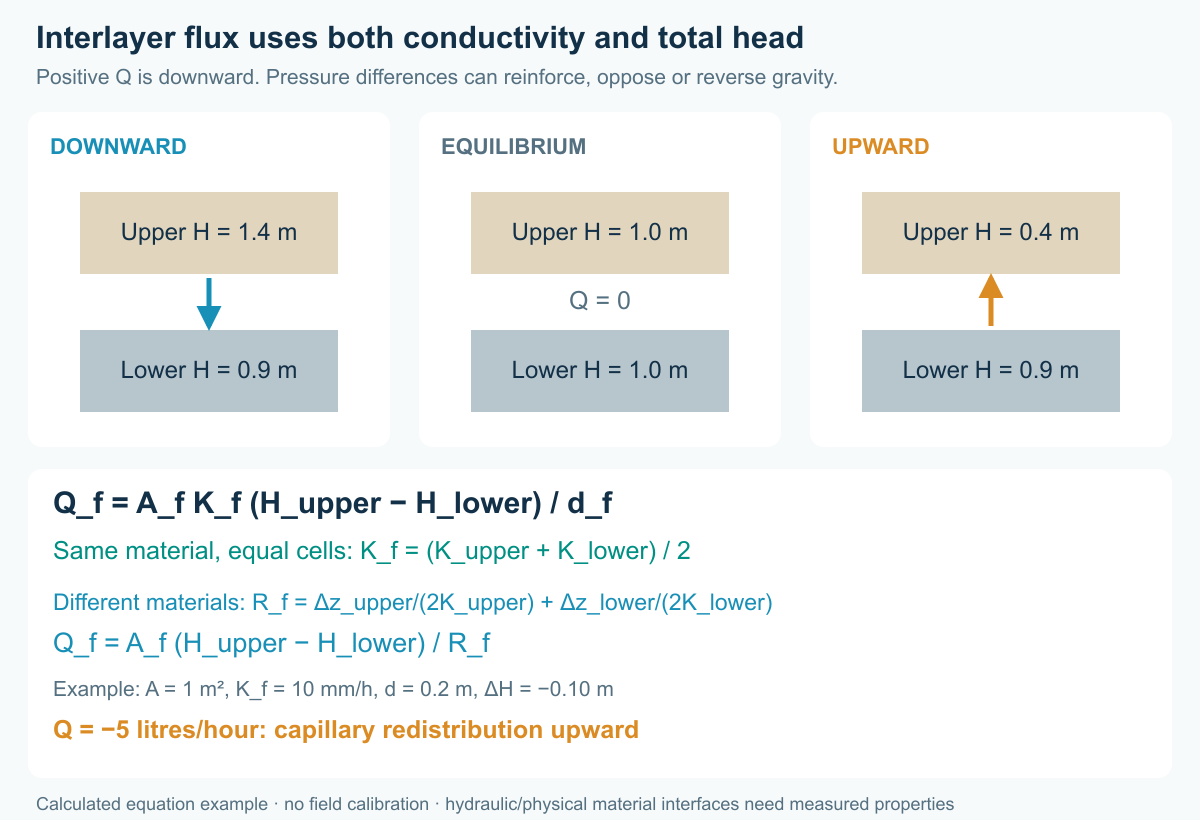
Figure 3. Signed Darcy–Buckingham flux at a cell face. Gravity and matric-pressure differences can reinforce or oppose each other; equal total heads give zero flux. Different-material interfaces use the combined half-cell resistance. Values are explanatory equation examples, not field measurements.

The spatial equations are integrated with adaptive BDF1 (implicit Euler). A full step and two half steps estimate temporal error, and the accepted update uses the two half steps. Newton iterations solve tridiagonal systems. Vertical integration and hydraulic routing are coupled in successive steps: boundary inputs remain fixed during a routing interval, then accepted port transfers are committed once. Cell-count, time-tolerance and routing-step sensitivity all matter; a small continuity error alone does not establish an accurate wetting-front position.

Local pressure connects the column to active controls

A buried link uses the total head of the cell intercepted by its port; a surface overflow uses ponding above its physical crest. For a fully submerged orifice without a flap gate:

Q = C_d Aₒ(u) sign(ΔH) √(2g |ΔH|)

The valve setting u controls the opening, while ΔH uses heads at both ends. Rising downstream head can suppress drainage or reverse flow. SWMM also handles partial wetting and structure-specific limits. EPA Hydraulics Reference Manual, Chapters 3 and 6.

Show static figure

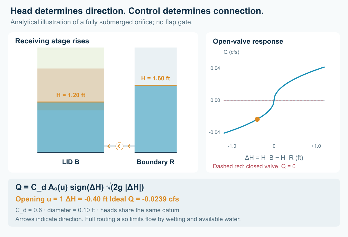
Figure 4. Analytical submerged-orifice illustration with a 0.10-ft opening and C_d = 0.6. It explains the mechanism rather than replaying the tutorial controller. Playback is slowed; the displayed heads and ideal discharge remain unchanged. Static figure.

Reverse inflow adds water to the intercepted porous cell. Its pressure changes through the storage law, and subsequent Richards fluxes redistribute that water through the column. A later storm therefore meets the resulting moisture/pressure profile, without clearing or reconstructing a Green–Ampt front. In Richards mode, node HEAD and DEPTH describe the surface reservoir, not a subsurface water table; inspect the cell pressure profile for buried-port conditions.

Show static figure

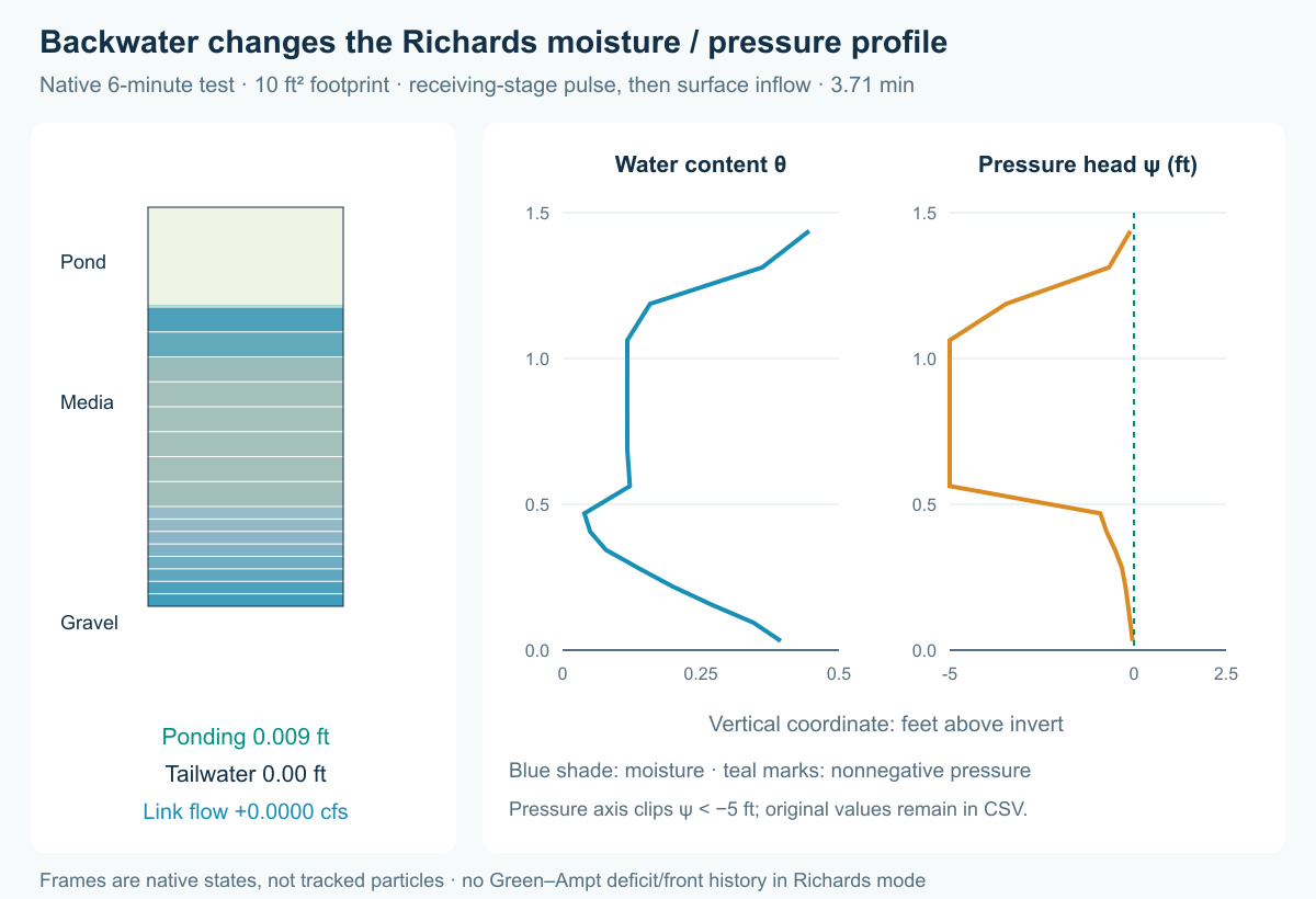
Figure 5. Native Richards pressure/moisture profiles in a separate six-minute backwater-and-second-event test. The diagram and time cursor come from sampled engine states; arrows indicate flow direction rather than tracked particles. This small fixture differs from the 24-hour chain. Static figure.

What is retained—and what remains simplified

This is a spatial approximation of the one-dimensional Richards equation, including the matric term; it is no longer the previous unit-gradient approximation. It assumes constant-density, isothermal matrix flow, a vertical column, atmospheric air pressure, local hydraulic equilibrium and single-valued retention/conductivity curves. Lateral unsaturated gradients, preferential/macropore flow, retention hysteresis and a resolved root-uptake field are not represented. Engineered media still require measured or defensible retention data. Richards can address matrix wetting, drying and capillary redistribution; that does not make every application more accurate without suitable parameters and discretization checks.

The existing model remains available when its reduced parameter demand and drainage approximation suit the question. More cells in that model refine its gravity-drainage balance; they do not add the missing matric term. EPA LID source.

Tu, Wadzuk and Traver (2020) represent gravity and matric-driven redistribution through connected, internally uniform blocks implemented with SWMM pumps and controls. Their diffusivity form uses D(θ) = K(θ) dψ/dθ, with moisture-to-matric-head conversion across textures. The new native column instead solves signed total-head fluxes directly between numerical cells and uses explicit interface conductances. Both retain the gravity and matric contributions of vertical matrix flow; their discretization, boundary treatment and calibration differ. The paper's HYDRUS comparisons are not validation of this native implementation. Tu et al., 2020.

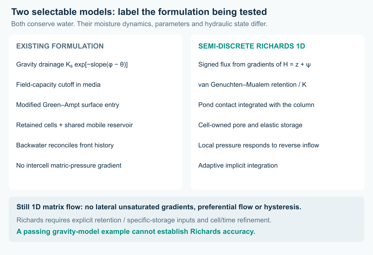
Figure 6. The optional models use different water ownership and constitutive laws. Their results must be labeled by formulation; a previously passing gravity-model test is not a Richards verification.

Treatment follows accepted directional water transfers

Each wet porous cell carries pollutant mass Mᵢ and concentration Cᵢ = Mᵢ/Wᵢ. An accepted transfer removes its donor concentration times the transferred volume, bounded by available mass, and credits the receiving cell after any authored-layer exit treatment. Surface ponding has its own mixed concentration. Evaporation removes water and retains solute. Standard pollutant advection follows the accepted directional water ledger; hydrodynamic dispersion, sorption and species-specific reactive transport are not added by selecting Richards.

For the first-order reaction update:

M_after = M_before exp[−(k_bg + k_layer) Δt]

Fixed removal acts once when water leaves an authored layer, rather than at every internal numerical face. A surface bypass does not inherit all buried treatment rules. The existing flow model retains its shared mobile-water reactor; Richards saturated cells keep their individual inventories. EPA Water Quality Reference Manual, Chapter 5.

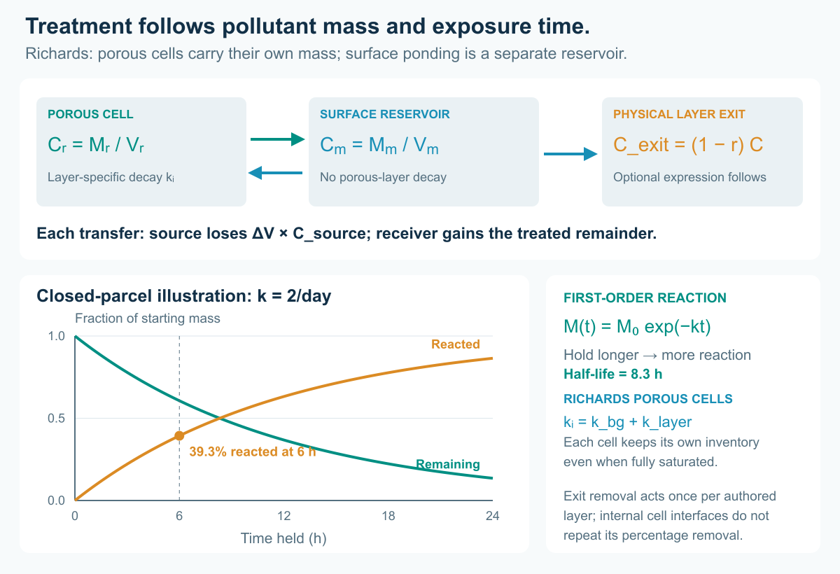
Figure 7. Closed-parcel decay with k = 2/day has a half-life of ln(2)/k = 8.3 hours. Longer exposure necessarily produces more modeled reaction under this assumption. The network determines exposure, bypass, release and remaining mass; this uncalibrated rate does not establish a field treatment mechanism.

Six small experiments with one common system

The accompanying tutorial uses two 1,000 ft² facilities, A and B, connected in series. Each has a six-inch surface layer, twelve inches of media and twelve inches of aggregate. Valve V_AB connects A to B; V_BR connects B to receiving boundary R. Separate emergency weirs connect each surface to an outfall, so bypasses remain visible in the assessment.

A two-hour triangular inflow peaks at 0.30 cfs and delivers 1,080 ft³ to A. It contains 20 mg/L of a conservative tracer and 20 mg/L of a hypothetical reactive constituent. The reactive constituent has a first-order rate of 2/day in each porous layer, with no fixed percentage removal. The specified porous-layer rate corresponds to a half-life of 8.3 hours; each Richards porous cell uses its layer rate, while surface ponding has no porous-layer reaction. This deliberately simple assumption isolates the effect of exposure time: longer exposure gives more reaction by construction. It is not a calibrated prediction for sediment, nitrogen or phosphorus.

For the backwater cases, R rises to a head of 1.60 ft. Reverse water is explicitly assigned zero pollutant concentration, making it a clean hydraulic boundary rather than an unreported pollutant source. Separate engine regression cases test both clean and held-concentration backflow.

The Richards head guard for V_BR closes above a receiving stage of 1.25 ft and holds until it falls below 1.05 ft. V_AB instead monitors B's surface HEAD at 2.25/2.05 ft: its media top is at elevation 2.0 ft, so these thresholds refer to 0.25/0.05 ft of ponding. The reopening band helps avoid rapid switching. A higher-priority depth-relief rule opens a valve above 2.20 ft only when downstream head is low. The emergency weirs remain available throughout. These are transparent test rules, not an optimized controller. In Richards mode, node HEAD and DEPTH track surface ponding, while buried links use their local cell pressure. These surface-based rules are intentionally distinct from the earlier mobile-water-table guards. Emergency overflow remains independent of controller operation.

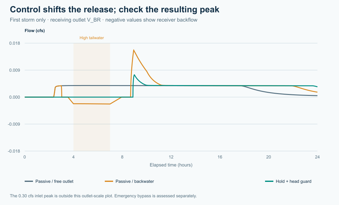
Figure 8. Receiving-outlet flow for the first-storm cases. Negative discharge represents backflow. The plot uses an outlet scale; the inlet peaks at 0.30 cfs. Emergency bypass is evaluated separately.

Comparing formulations, with explicit limits

The gravity/front results above were rerun after correcting the retained/mobile partition bug described below; the earlier comparison values are withdrawn. This column uses legacy exponential drainage and Green–Ampt entry. Richards adds explicit, uncalibrated retention/specific-storage properties and has different initial water ownership; the inter-facility head guards also use surface-ponding thresholds. The routing steps differ and are identified in the table. These are illustrative configurations, not a calibrated equivalence experiment or proof that either formulation is superior. The Richards grid/timestep sensitivity below limits quantitative comparisons.

Longer detention can help treatment—and change the risk

The tracer timing is the elapsed time when sampled discharge through all three outfalls has exported half of the event's input tracer mass. It is not a mean residence time or a residence-time distribution. Reported reaction percentages use the engine's cumulative mass budget at 24 hours.

The tendency for longer exposure to increase reaction follows directly from the assumed first-order decay law. The experiments assess how network hydraulics and controls change exposure, export and inventory. They do not independently establish a field treatment benefit. In the illustrated Richards runs, holding changes release timing and modeled reaction, but does not guarantee a smaller receiving-outlet peak. Count emergency bypass and stored mass alongside controlled discharge.

These Richards examples are diagnostic experiments, not an optimized design or a converged ranking of controllers. The cell-count and routing-step checks below show why a richer equation must be accompanied by numerical verification. Other storms can also shift a delayed release into another tributary’s peak. Active control requires a system objective—such as pollutant export under a downstream flow limit—together with explicit accounting for bypass and available storage.

Show static figure

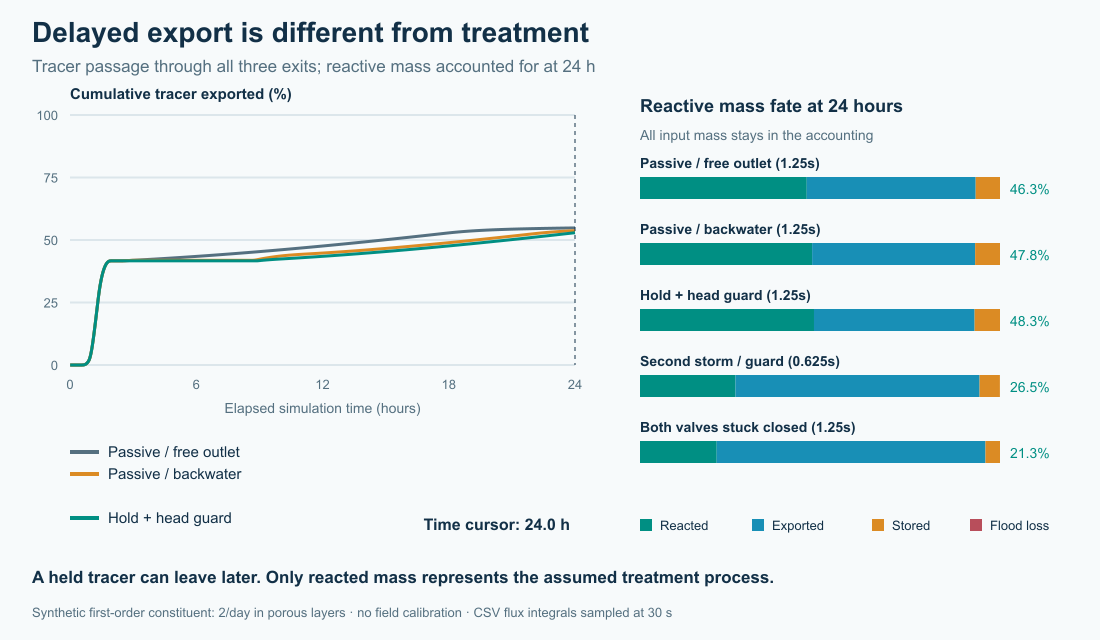
Figure 9. Curves progressively reveal cumulative tracer export from sampled link flows and concentrations. The adjacent bars always show the final 24-hour reactive-mass budget (second-storm step 0.625 s; other displayed strategies 1.25 s); they are not time-varying inventories. All exits and any flooding loss are included. A low export at an intermediate time can mean temporary storage. Static figure.

The repeated-storm and stuck-valve cases make that distinction concrete. A zero controlled-outlet flow does not mean zero discharge to the environment. Emergency overflow and flooding can carry pollutant out, while an inventory remains in the facilities. Count every destination before reporting cumulative treatment. In the corrected two-storm guarded case, the engine records approximately 1,743 ft³ of emergency-weir discharge; with both valves stuck closed, that volume rises to approximately 2,016 ft³. Neither case has a flooding loss in these runs. The emergency weirs drain perched surface water at the intended crest. These totals are from the Richards runs. These cumulative totals include brief overflows that coarse snapshots can miss.

A pollutant balance before a performance claim

For each constituent, the assessment checks:

Initial mass + incoming mass = discharged mass + flooding and seepage losses + reacted mass + final stored mass.

Storage includes all porous-cell and surface inventories, including elastic water in the Richards saturated branch. In a reversing system, incoming mass includes any pollutant carried from the receiving boundary. Concentration alone is insufficient: exported load depends on integrating flow multiplied by concentration over time. The EPA Water Quality Reference Manual describes SWMM's pollutant routing and treatment framework.

Developing these tests exposed two accounting problems: returning boundary pollutant was not booked as an external source, and a nearly dry LID could lose the load of water that percolated and drained during the same routing step. The correction carries the same accepted transfer concentration to the donating and receiving compartments, resolves the connected mobile mixtures consistently and books treatment once. Overflow ports also use their physical weir crest when selecting the supplying layer. A separate roundoff error at a nonzero node invert could place a crest intended at the surface/media interface in the media cell, causing the weir to miss perched ponding. Corrected elevation arithmetic and a shared, roundoff-tolerant interface rule now select the intended head, water source and pollutant treatment layer.

The six examples were run with Richards explicitly enabled. The first four illustrated strategies use eight cells per porous material and a common 1.25-second fixed routing step; the second-storm figure uses 0.625 s and the stuck-closed case 1.25 s. The publication package contains 14 checkpointed complete case/numerics combinations, including finer routing, 4/16-cell and tighter ODE-tolerance checks. All these completed runs passed the 0.5% water/tracer/reactive continuity criterion without engine warnings; maximum reported error was 5.03e-11%. The two-storm case failed at 1.25 s with a Richards adaptive-step-limit error; it is retained as a failed check, not counted as a pass. The pressure-profile fixture passed at 0.1 and 0.05 s. These are not numerically converged performance predictions: routing-step and cell-count changes materially affect outlet peaks, reverse volumes and treatment exposure. The recorded Richards publication verification passed 9 kernel tests and 49 of 50 LID-node integration tests; the US/SI storage-equivalence fixture remains failing. The older 241-test/20-run evidence applies to the previous gravity/front implementation, not Richards.

The grid dependence is large enough that these runs cannot establish a robust ranking of control strategies. The guarded case’s tighter ODE tolerance changes reacted fraction by 0.000 percentage points; this does not resolve the distinct cell-size/routing coupling sensitivity. Further numerical verification and measured retention properties are needed before design use. The 02_passive_backwater peak changes from 0.0155 to 0.0199 cfs at 0.625 s. The 04_head_guard peak changes from 0.0074 to 0.0115 cfs at 0.625 s.

A small water-balance error alone is not sufficient evidence of correct pollutant routing. We check a conservative tracer, the reacting constituent and routing-step sensitivity before interpreting treatment. The supplied kinetics, footprints, conductivities, storm pulses and boundary stages remain illustrative. Field applications require site data and pollutant-process calibration.

Independent testing identified another problem in the earlier gravity/front model: an inlet above the reported water table could keep filling a partially submerged cell as retained moisture, while that cell stopped free drainage as soon as its bottom was submerged. At porosity, its remaining mobile capacity collapsed and its water inventory was abruptly reclassified. Water was conserved, but the resulting head and hydrograph were wrong. The reproduced free-outlet case rose 0.993 ft in 30 seconds while total water fell from about 517 to 514 ft³; the backwater case rose 0.631 ft at about hour 2.675. The correction keeps partially submerged cells draining retained excess and routes incoming water to mobile storage when the receiving cell intersects the water table, even if its inlet is above that table. Only fully submerged cells skip free drainage. This is the reduced model’s cell-level coupling approximation, not a resolved local Richards pressure field. After correction, the largest 30-second rise in B is about 0.0031 ft in both examples, and the free-outlet case no longer has the artificial reversal into A. All six legacy examples passed water/tracer/reactive balances at 0.5 and 0.25 s (12 completed runs); the current LID-node suite passes 52 of 53 tests, including three new regressions for partial-cell drainage, inlet ownership and per-step routed-head continuity. The previously reported Richards US/SI fixture still fails. These results replace the affected legacy performance comparison; the Richards figures retain their separately identified run provenance. Continuity is necessary, but head continuity and a physically consistent storage partition must also be checked.

Configure the same example in SWMMVis

Open richards_04_head_guard.inp from the Richards example bundle. Inspect storage A or B: LID Control is Train and LID Initial Saturation (%) is 10. Open Model → LID Control, select Train, and choose Richards 1D under Flow model. The two authored porous layers remain MEDIA and AGGREGATE; numerical subdivisions are configured separately.

Under Physical properties, verify the thicknesses, porosities and saturated conductivities, then enter the explicit retention properties:

These are illustrative properties, not a conversion from the older conductivity slope. Alpha and specific storage remain in inverse metres even though this CFS project displays thickness in inches and conductivity in inches/hour. Expand Numerical settings: use 8 numerical cells per porous layer, absolute water-content tolerance 1e-7, relative tolerance 1e-5, and maximum internal step 30 s. Inspect the moisture/conductivity curve preview.

Under Pollutant treatment, assign REACTIVE to each porous layer, set Removal (%) = 0, Decay (1/day) = 2, and leave Expression empty. Use Apply layers and treatment and save. Set a fixed routing step of 1.25 s for the four first-storm strategies and the stuck-closed case, and 0.625 s for the second-storm case; use variable-step factor 0. The download copies already carry these tested steps. The validation companion reports routing, cell-count and ODE-tolerance checks, including the failed second-storm run at 1.25 s.

Inspect V_BR's layer-3 bottom anchor, both surface overflows, and V_AB's explicit offsets. Review the surface-HEAD thresholds in Model → Data Objects → Control Rules…. Run the six files separately, compare all signed flows and mass destinations, and inspect the live section's numerical-cell moisture/pressure. Saved profile time histories are pending; the figure runner records the live API explicitly.

The T10 tutorial supplies the complete workflow. Download the six Richards models and short profile fixture; the original gravity/front examples remain available for a clearly labeled comparison. Richards hotstart extension 11 preserves complete cell water and material identity. Runtime aquifer-bed exchange, water age, heat and MSX are not yet supported with Richards nodes.

From distributed LIDs to receiving waters—and groundwater

The larger objective is to move from discrete LID performance to the system-wide implications of distributed LIDs for receiving water bodies: event peaks, delayed releases, cumulative loads and the pathways connecting facilities across a watershed.

The new spatially explicit groundwater model extends that perspective below the surface. Its mesh-based two-zone representation supports spatial aquifer properties, lateral groundwater flow, recharge, saturation-excess return to the surface and configurable exchange with drainage infrastructure. It provides a basis for asking where infiltrated water travels and when it returns to the drainage network or receiving waters. The demonstrations use a closed bottom boundary. The Richards LID–aquifer bottom-interface adapter remains pending, so these runs do not demonstrate coupled groundwater exchange or groundwater pollutant treatment.

Future articles will explore that connection: distributed recharge and changing water tables, surface-water–groundwater feedbacks, and how those pathways alter the combined benefits and constraints of LID placement and active control. The question is becoming what the distributed system delivers to the receiving water, over time.

Acknowledgments

I thank Dr. Rob Traver for discussions that helped refine the ideas behind the LID Storage node implementation and for his support of its development and implementation. I also thank Corinne Wiesner-Friedman and Robert Dickinson for reviewing this article.

Acknowledgment of AI assistance

OpenAI Codex assisted with drafting and editing this article and developing the scripts used to create its figures and GIF animations. The network performance results come from the documented SWMM simulations; the formulation diagrams and orifice animation are explanatory illustrations. Caleb Buahin is responsible for the technical interpretation and final content.

References

• Ireson, A. M., Spiteri, R. J., Clark, M. P., and Mathias, S. A. (2023). A simple, efficient, mass-conservative approach to solving Richards' equation (openRE, v1.0). Geoscientific Model Development, 16, 659–677. Published paper.
• U.S. EPA (2018). SWMM Build 5.1.013 release notes, underdrain control additions. EPA release notes.
• U.S. EPA (2022). Storm Water Management Model User's Manual, Version 5.2. EPA/600/R-22/030. EPA manual.
• U.S. EPA. SWMM solver source: LID fluxes and infiltration. lidproc.c; infil.c.
• Rossman, L. A. (2017). Storm Water Management Model Reference Manual, Volume II: Hydraulics. EPA/600/R-17/111. EPA hydraulics reference.
• Tu, M.-c., Wadzuk, B., and Traver, R. (2020). Methodology to simulate unsaturated zone hydrology in Storm Water Management Model (SWMM) for green infrastructure design and evaluation. PLOS ONE, 15(7), e0235528. doi:10.1371/journal.pone.0235528.
• Rossman, L. A., and Huber, W. C. (2016). Storm Water Management Model Reference Manual, Volume III: Water Quality. EPA/600/R-16/093. EPA reference.
• Sharior, S., McDonald, W., and Parolari, A. J. (2019). Improved reliability of stormwater detention basin performance through water quality data-informed real-time control. Journal of Hydrology, 573, 422–431. doi:10.1016/j.jhydrol.2019.03.012.
• Gomes Junior, M. N., Giacomoni, M. H., Taha, A. F., and Mendiondo, E. M. (2022). Flood Risk Mitigation and Valve Control in Stormwater Systems: State-Space Modeling, Control Algorithms, and Case Studies. Journal of Water Resources Planning and Management, 148(12), 04022067. doi:10.1061/(ASCE)WR.1943-5452.0001588.

What built-in shape tables get wrong, what replaces them, and what it costs

Where this started

I am building an uncertainty sidecar slowly for SWMM on a different branch (I am super excited to post about that down the road). It has me constantly wondering about uncertainty that exists in SWMM that I may overlook. I started to think about SWMM's look up tables, which are approximations of pipe shapes. I was thinking, well, how much error might this account for and under what conditions? What might this mean for pipe Manning's? When we calibrate this, are we just calibrating something that may very well just be an error term? In particular, how might this affect the finite volume solve?

I started investigating this and after realizing that pipe geometry has bigger implications to a finite volume solver, I ended up pursuing work from the practical perspective of finding an approach that would reduce that error and let people input any hollow pipe shape they want.

I have really enjoyed reviewing some math I kind of knew and deepening my understanding of it in application to this work.

What follows is an AI-written summary that I directed and verified about what turned up and some of what it implies.

Maybe this will spark your interest if you have a network with some funky shapes. I hope you try out these new features, help debug a bit, and get back to me on how your results may have changed.

— Corinne Wiesner-Friedman

Five-minute version. SWMM describes each built-in pipe shape with two small lookup tables that contradict each other: differentiate the area description and you do not get the width table back. That is not a precision problem. The equations these solvers integrate assume top width is the derivative of area, so an inconsistent pair means the solver is being handed a cross-section that cannot exist. We replaced the tables with exact geometry, which fixes that by construction.

The finding worth your attention is what happened next: switching to exact geometry moved dynamic-wave hydrographs — a median of 7% of peak flow at each conduit's worst moment, 1.2% averaged over the whole record — while the continuity error stayed flat at ~0.08%. The model's standard quality check is structurally blind to this class of error. Peak values themselves barely moved, which is a finding in its own right. Everything below expands on that, and every claim links to the code or the measurement behind it.

Continuity stayed flat while the predictions moved

Both panels are the same two runs: Bellinge (1015 conduits, 48 h, dry-weather), dynamic wave, one binary, one changed option — XSECT_GEOMETRY LEGACY versus EXACT.

Left: what the model says about its own quality. Continuity error moves from 0.073% to 0.085%. By that measure, nothing happened.

Right: what the model actually computed. Take each of the 189 conduits carrying more than 1 L/s and ask how far apart the two flow records ever get, as a fraction of that conduit's own peak: 80% diverge by more than 1% of peak at some point, 45% by more than 10%, and 33% by more than 25%. Median 7.0%; averaged over the whole 48 h rather than taken at the worst instant, the median is still 1.2% and the upper decile 14%. Node depths behave the same way (median 5.8% at the worst instant; one node's depth differs by 755 mm at one moment).

What does not move is the peak. Peak flows agree to a median of 0.20%, and the largest change in any node's peak depth across the whole network is 2 mm. So exact geometry does not rescale the answer — it shifts the timing and shape of the hydrograph underneath an almost unchanged peak. That distinction matters if you calibrate to peaks, and it matters more if you use the model for anything that integrates over the record: first flush, pump cycling, CSO spill duration, sediment transport.

Same water, same network, same solver, same time-step settings. The only difference is how the pipe's cross-section was described.

The uncomfortable implication. A modeler checking continuity to decide whether a run is trustworthy would see no reason for concern in either run. The error is real, it is systematic, and the standard diagnostic cannot see it. That is what "unquantified uncertainty" looks like in practice — not a missing error bar, but a quality check pointed at the wrong quantity.

The area and width tables describe different pipes

SWMM describes each shape's area and its top width with separate, independently digitized tables — and for four shapes the area description is itself a second table, inverted. But width is the derivative of area; they are not independent facts. Differentiate the area description and you should recover the width table. You do not.

A 2 m gothic sewer holding 2% of its capacity. Gothic is one of the shapes that ships no area table, so its area comes from a 51-point depth-of-area table instead: read that, and the water surface is at 0.090 m. Integrate the shape's own 21-point width table to the same stored volume and it is at 0.146 m. The orange band is the 56 mm the two descriptions cannot agree about — drawn at true scale. At 0.5% capacity the two answers are 23 mm and 74 mm — more than a factor of 3.

A LEGACY run consults both tables in the same timestep — area from one, width from the other — so the disagreement propagates into surface storage, friction and wave speed continuously.

The disagreement is worst where models spend dry weather, and it is much worse for some shapes than others:

Two notes on reading that table. The 2% depth column is a local slope, so it is sensitive to where the table's own nodes fall: y/D = 0.02 is exactly a node of circular's 51-point table, and the slope jumps from −34% just below it to +22% just above, which is why that cell carries two numbers. Every other row sits mid-interval and is a single value. The last two columns are dense sweeps and are not node-sensitive.

The pattern is not random: of the eight shapes here, the four worst are exactly the four that ship no area table at all. Those four carry only a 21-point width table plus 51-point depth-of-area and section-factor tables, and their area is recovered by inverting the depth-of-area table (XSectKernels.hpp) — a second, independently digitized description of the same pipe, which is exactly why it need not agree with the first. Circular — the best-resourced shape, and the one most networks are mostly made of — is by far the best behaved. (The pattern is suggestive rather than a law: HORIZ_ELLIPSE, which is not in the table above and does ship a 26-point area table, computes to a comparable ~12% median.)

Why this is a correctness problem, not just a precision one. The Saint-Venant equations are not agnostic about geometry — they are derived assuming a real cross-section. Continuity is ∂A/∂t + ∂Q/∂x = q, and writing it in the depth form every solver actually uses requires the chain rule step ∂A/∂t = T·∂y/∂t — which is valid only if T = dA/dy. Give the solver a T that is not the derivative of its A and the discrete system is no longer a discretization of the shallow-water equations for any pipe. It is a discretization of an inconsistent system.

This is not abstract. Dynamic wave uses top width to convert net inflow into head change at a node (surfArea = (w1 + wM)·length/4, DynamicWave.cpp) and area to report the volume stored in the conduit (links.volume = area_mid · length · barrels). Those are precisely the two tables that disagree. No physical cross-section has gothic's tabulated area and its tabulated width — so the pipe the momentum equation sees and the pipe the continuity equation sees are different objects.

Exact geometry does not merely reduce this error, it removes its cause. Area and width stop being two digitizations and become two boundary integrals of one and the same outline, on which T = dA/dy holds identically. What the solver evaluates is a compiled approximation of that outline, so the identity survives to the fit tolerance rather than to the last bit: measured on a compiled 4 ft circle, |dA/dy − T|/T has a median of 1×10⁻⁸ and a worst case of 1.5×10⁻⁷. The circular tables it replaces, measured the same way over the same depth window, sit at 0.6% median and 22% worst — six orders of magnitude apart, and circular is the best of the shapes.

Dig deeper. The constants themselves: xsect_tables.hpp. The inherited-defect register, including this one as LD-1: docs/dev/legacy_defects.md. Reproduce the table above by resampling both descriptions — the area table where one exists, the inverted depth-of-area table where it does not — scaling by each shape's aFull/wMax from xsect.c, differentiating the area, and comparing to the width table.

Only finite volume converts a geometry error into a mass error

The same geometry error sits in both solvers. Only one of them has an instrument that detects it.

• Dynamic wave consults geometry. It asks for an area at a depth and uses the answer. The error perturbs that timestep and leaves no trace in any mass balance.
• Finite volume embeds geometry in its conservation statement. Cell state is flow area; depth is recovered by inverting the same geometry every substep. A geometry inconsistency becomes a mass error — and mass errors show up on the continuity line.

Read this the right way round. FV's large continuity error under LEGACY is not evidence that FV is worse — it is evidence that FV can see something DYNWAVE cannot. The dynamic-wave row looks clean not because its geometry is accurate, but because it has no mechanism that converts geometry error into mass error. The figure at the top of this piece is what that same error looks like when you go and measure it directly instead of trusting the diagnostic.

The reason is worth stating plainly, because it is structural rather than incidental: DYNWAVE's continuity check balances volumes that are themselves computed from the geometry in question. Stored conduit volume is area × length, read from the same area table that drives the routing. A geometry error therefore shifts both sides of the ledger together and the balance still closes. The check confirms the bookkeeping is self-consistent; it was never an instrument for asking whether the geometry is right. FV, by contrast, must invert its geometry every substep to recover depth from the conserved area — so an inconsistency has nowhere to hide.

For the numerically inclined. The requirement FV imposes is stated in FvKernels.hpp: the composition depthOfArea ∘ areaOfDepth must be the identity, not merely accurate, or cells at equal free surface but different bed elevation reconstruct different surfaces and lake-at-rest fails. Two independently digitized tables cannot satisfy that. One boundary can, by construction.

One exactly integrated boundary replaces the tables

Draw the pipe's real boundary as straight segments and circular arcs. Compute its hydraulics from that boundary once at load time via Green's theorem — a closed-form contour integral, so at any depth the area, perimeter and top width are exact, with no depth table and no linear interpolation anywhere. Then compress those exact functions into a piecewise polynomial the solver evaluates in a short chain of multiply-adds.

The property that matters is that every quantity now comes from one object. Area, top width, perimeter, hydraulic radius and section factor are five quantities computed from a single outline rather than five separately digitized tables, so they cannot describe different pipes — T = dA/dy holds identically. The compiled polynomials inherit the identity to about 10⁻⁸ relative, six orders tighter than the tables, rather than the exact zero the underlying geometry has.

The mathematical core, for those who want it. The area-versus-depth curve kinks where the surface crosses a corner and picks up a square-root branch point where it goes tangent to a curved wall. Split the depth range at those critical heights and each piece is analytic — where polynomial approximation converges geometrically (Trefethen, Approximation Theory and Approximation Practice, Chs. 3 and 8). The critical heights are the critical values of the height function on the section's boundary — Morse theory in the textbook sense where the wall is smooth (Milnor, Morse Theory), with corners and flat crowns contributing critical heights of their own; the height has no critical points in the interior, and the piecewise structure is a Reeb graph on the depth axis (Edelsbrunner & Harer, Computational Topology, Ch. VI). A per-piece change of variable removes the branch points. Implementation and convergence argument: docs/dev/cheb_section.md, ChebSection.hpp, XSectBoundary.hpp.

Arbitrary and time-varying sections become expressible

POLYGON takes an explicit boundary of lines and arcs

POLYGON takes an explicit boundary of lines and arcs — asymmetric, benched, filleted, surveyed. It is evaluated exactly, and a bench's top-width jump is represented rather than smoothed away.

Worth being precise about what "open channel" means here, because it is not what you might assume. The outline you supply is always a closed chain — it has to be, since the exact area and perimeter come from a boundary integral around it, and a self-intersecting or dangling chain is rejected with an error. A separate flag in [XSECTIONS] (Link POLYGON Scale Open 0 0 Barrels Bcurve) then declares whether the top of that outline is a wall or a water surface. Set it open and the top edge drops out of the wetted perimeter, conveyance stays single-valued, and water rising past the drawn section extends it with vertical walls rather than pressurizing through a Preissmann slot. So you draw a closed shape and tell the engine whether its lid is concrete or air.

This matters because the existing escape hatches are narrower than they look. IRREGULAR is open-channel only, so it cannot close over a box culvert. CUSTOM is closed but symmetric — a width-versus-depth curve says how wide the water is, not where the walls are, so it cannot express a one-sided deformation, and friction is then computed against an assumed shape. Both are resampled into fixed 51-point interpolated tables, reintroducing exactly the error described above: the CUSTOM table carries about 41% area error below 5% of full depth.

Dig deeper. [XSECTIONS] and [CURVES] XPOLYGON syntax with a worked four-arc circle: AppendixD.md. Boundary construction and validation: XSectBoundary.cpp.

A conduit's section can be replaced between routing steps

swmm_link_set_polygon() replaces a conduit's cross-section between routing steps, and the solver reconciles the water already in the cells. This is the piece that makes sediment, relining and progressive narrowing modellable as processes rather than as separate scenarios.

The caller states which physical event it is, and there is deliberately no default, because the two cases are opposites:

One counter-intuitive detail worth knowing: a sediment bed is not simply a smaller pipe. A flat bed in a round invert is wider at the water line than the invert it buried, so a silted conduit can hold more water at a given depth above the bed. The engine tracks bed level separately and preserves free surface elevation, not depth — without that, adding sediment reads as adding capacity.

Mid-run changes currently require the FV solver; the legacy solvers accept a new section before a run starts but not during one.

Dig deeper. Policy semantics and the displaced-volume contract: INetworkSolver.hpp. C API: swmm_link_set_polygon.

EXACT costs about 1.6× on this network, and part of that is a build flag

Those are whole-run wall times for one binary on one machine, and part of the gap is not geometry at all. The engine is built with -ffp-contract=off, which forbids the compiler from folding a×b + c into a single fused multiply-add. The flag is there to enforce the legacy bit-parity contract: with fusion allowed, the same expression rounds differently depending on which call site it was inlined into, which was enough to break several exact-equality tests against EPA SWMM 5.2.4 (src/engine/CMakeLists.txt).

That flag does not fall equally on the two modes. Evaluating a Chebyshev series is almost nothing but alternating multiplies and adds — exactly the pattern fusion exists to accelerate — whereas a table lookup is mostly a bounds check, an index and one interpolation. So the compiled path is structurally the more exposed of the two, and some share of the ratios above is the price of reproducibility rather than the price of geometry. We have not measured that share. Doing it credibly means building the engine both ways and interleaving the runs; this machine has shown up to 18% run-to-run spread on this benchmark, so an uncontrolled before-and-after would not settle it. Treat the 1.58× and 1.68× as what they are — the cost of the shipped build — and the split between "geometry" and "reproducibility" as open.

Why we are not telling you to just switch fusion on. Two reasons, and the second is the one that surprised us. LEGACY mode lives in the same engine target — it is the v6 engine reproducing EPA's numbers — so enabling fusion globally would strip the parity guarantee from LEGACY runs in that build, and scoping it to the compiled-geometry translation units alone leaks through header inlining. And FV is not the free case it appears to be: FV sits outside the parity contract by design, but it is an explicit substepping scheme in which any bit-level change compounds, and the engine's own build notes record a contraction change moving ~26% of FV output values and the continuity error from −2.989% to −3.124%. Being outside the parity contract means those differences are not guaranteed to be zero; it does not mean they are negligible.

Per shape the picture varies in both directions. Gothic is 5.6× faster compiled, because its legacy path has no area table and must reconstruct one. Circular is the worst case at ~1.15× slower — and it is computing a fourth quantity for that price. Both are per-call microbenchmarks from an earlier build, not extracted from the whole-run times above.

A caution on generalising from Bellinge. Of its 1031 cross-sections, 953 are circular and the other 78 are shapes EXACT does not compile at all. So the entire cost and the entire benefit above are the same 953 pipes. We confirmed this directly: restricting EXACT to every shape except circular produces output byte-for-byte identical to LEGACY. Bellinge cannot tell you what exact geometry is worth on the shapes it helps most, because it contains none of them.

That points at a third mode we have not built — call it SPEED — which would compile a boundary whenever doing so is faster, regardless of accuracy. The dispatch is already per link, so this is a policy, not new plumbing. It would match EXACT on gothic-family shapes (faster and more accurate, no trade) and diverge on circular, leaving it on the table. Honest caveat: only circular and gothic have measured per-shape runtimes; the nine other shapes EXACT compiles are inferred from structure, not timed.

What this does not show

• No validation against measurement. Everything here is measured against exact geometry, the tables' internal contradictions, or the model's own mass balance — never against observed flow or level. The defensible claim is "the geometry is demonstrably more correct," not "the model is more accurate."
• The DYNWAVE differences above are not an error bar. They measure how far the answer moves between two geometry representations. Since EXACT is demonstrably closer to true geometry, that spread is a reasonable estimate of what LEGACY carries — but it is a difference, not a validated uncertainty.
• The differences are in the hydrograph, not in the peak. Peak flows and peak depths are essentially unchanged on this network. Anyone whose interest is peak magnitude should read the result as "geometry error was not distorting your peaks here", not as a warning about them.
• "Exact" is qualified for most shapes. Circular and POLYGON are genuinely exact. The other tabulated shapes are reconstructed from their own 21–26-point width tables, so EXACT gives them internal consistency, not new information. Gothic results will move noticeably.
• One network, one machine, dry weather. Bellinge is mostly circular. Wet weather, surcharged conditions and other shape mixes are untested.

The correctness claim is settled; the predictive claim is not

We set out to let SWMM represent pipes it could not draw. We found that the shapes it can draw are described by tables that disagree with each other, in one case by more than the quantity they describe — which means the governing equations have been integrating a cross-section that does not exist.

Two things follow, and they are different claims. The correctness claim is settled and needs no field data: exact geometry makes T = dA/dy true by construction, so the solver is finally solving its own equations for a real pipe. The predictive claim is not settled — whether that produces better forecasts depends on calibration absorbing the old bias, and we have not tested it against observations.

The result worth carrying is the one in between: the model's standard quality check did not notice either way. Continuity stayed at ~0.08% while a third of the meaningful conduits saw their flow record diverge by more than a quarter of their own peak at some point in the run — even though the peaks themselves barely moved. Whatever else exact geometry is worth, it has made visible a source of uncertainty that has been in every dynamic-wave run for half a century with no diagnostic pointed at it.

XSECT_GEOMETRY EXACT is opt-in and alpha; LEGACY is the default and its output is byte-for-byte unchanged. Full technical detail is in the feature/xsect-geometry → swmm6_rel pull request (39 commits). The legacy solver in src/legacy/ is unmodified.

Reproducing the top figure: run Bellinge twice under DYNWAVE changing only XSECT_GEOMETRY, then compare the two .out files with scripts/compare_results.py's reader, over every reporting period rather than a subsample, restricted to link indices below the conduit count. Figures 2 and the shape table come directly from the shipped constants, independently of the engine build.

Open-Source SWMM's new finite volume routing engine: exact mass accounting, resolved flow regimes, and virtual junctions for all-pipes models. (Edited to fix typos)

Two surge-and-drain cycles over 24 hours in Cedar Glen, a synthetic 387-pipe raw-water conveyance built the way real GIS exports look: a 4.9-mile trunk drawn as hundreds of short survey segments, chained by virtual junctions, ending at a flow-regulating storage basin. The profile is drawn at true scale, and the numbered dots on the map mark the profiled trunk chainage. One input deck runs both solvers, and both carry a Preissmann slot above the crown: blue is the new finite volume solver, green dashes are dynamic wave with its own slot option (SURCHARGE_METHOD SLOT), and the thin companion lines are each solver's energy grade line.

For over fifty years, SWMM has answered how much water a drainage system carries, its velocities, hydraulic grade lines, etc. These questions become harder to answer at the extremes. How do these attributes behave when the pipes go through filling and emptying cycles? Does the mathematics still add up in those moments? Those are relevant for designing conveyance systems and are exactly the places where classical solvers run into trouble. We have added an alternative solver to the legacy dynamic wave solver to Open-Source SWMM, using an explicit finite volume approach to make results at these extremes more trustworthy.

Mass Balance Errors are Now a Thing of the Past

The legacy dynamic wave solver iterates node heads and checks continuity after the fact; the report card tells you how much water went missing. The finite volume (FV) solver moves water between short cells as fluxes. Whatever leaves one cell enters the next, exactly, by construction, so conservation holds to machine precision at every step.

On Thacker's oscillating flat-bottom basin (Thacker, 1981) from the SWASHES analytic suite, dynamic wave manufactures a continuity error of -4,459 %. The FV solver reports 0.0 %. On three pressurization benchmarks built for exactly the regime where sewers get harder to simulate, FV closes to within 0.001 % on all three while the legacy surcharge iteration leaks 6.1 % of its throughput in a single surcharge cycle, and the leak grows as the mesh is refined (3.1 % at 20 m cells, 6.1 % at 5 m). Across the 20 models of EPA's dynamic wave quality assurance corpus (Rossman, 2006), FV routing continuity never exceeded 0.015 %, and on most models it reads exactly zero.

Finite volume solver closes to 0.001 % or better on all three. Dynamic wave is shown with its default EXTRAN surcharge accounting, its most stable configuration on these decks; its slot variant loses orders of magnitude more volume at the suite's fixed parity time step.

Flow Regimes the Legacy Solver Cannot Capture

The legacy dynamic wave solves one momentum balance per pipe and knows depth only at pipe ends. The FV solver subdivides every conduit into cells and solves the full shallow-water equations with a shock-capturing scheme, so backwater curves, chokes, bores, and hydraulic jumps live inside the pipe, at the station where they physically occur.

The SWASHES analytic benchmarks (Delestre et al., 2013) make the differences visible. In transcritical flow over a bump, the flow accelerates through critical depth at the crest and runs supercritical downstream. The channel is modeled 12 m deep so the case stays purely open channel and nothing constrains either solver. The FV solution converges to the analytic profile through the choke and down the supercritical branch, with an L1 depth error of 0.034 m and zero drift over the final five minutes. Dynamic wave never finds a steady state on this case: the upstream water surface sloshes between dry and more than 10 m deep for the whole run, and even its time-averaged profile sits 1.6 m from the analytic solution.

(SWASHES 3.1.4, Delestre et al. 2013). Both solvers get the identical deck: a constant 1.53 m³/s inflow upstream, a free downstream outfall, a frictionless bed, and a 12 m deep channel so the case stays open channel throughout. The finite volume solution is steady and passes through critical depth at the crest onto the analytic supercritical branch. Dynamic wave never reaches steady state here; the dashed line is its time-averaged surface and the shaded band is the range it sweeps through the second half of the run.

Where the flow comes back down, the difference is just as sharp. In MacDonald's 1,000 m benchmark channel (MacDonald et al., 1997) the bed is constructed so the steady solution jumps from supercritical to subcritical exactly at mid-channel. The FV solver holds the hydraulic jump as a discontinuity at x = 500 m with an L1 depth error of 2 mm. Dynamic wave finds the right depths away from the jump and smears the jump itself across more than a hundred meters of channel; its L1 error is 13 mm.

A steady hydraulic jump (MacDonald et al.1997; SWASHES 3.2.1, Delestre et al. 2013), shown as the full water surface profile over the constructed bed. In the inset, the finite volume solver drops onto the supercritical branch and holds the jump sharp at its analytic station; dynamic wave smears the jump across more than a hundred meters.

Ritter's dry-bed dam break (Ritter, 1892) tells the same story in a transient. The FV front tracks the analytic rarefaction smoothly to the wetting front (L1 error 0.020). Dynamic wave oscillates violently through the wave and cuts the front off early (L1 error 0.104).

A dam break onto a dry bed (Ritter 1892; SWASHES 4.1.2, Delestre et al. 2013). The finite volume profile follows the analytic solution through the front; dynamic wave rings through it.

Pressurization Physics

The transition from open channel to pressurized flow is one of the areas where storm sewers earn their keep and where solvers show their character. Both engines can carry a Preissmann slot (Preissmann, 1961) above the crown, so the fair comparison is between the two implementations.

In legacy SWMM engine, the slot is an option alongside the default EXTRAN surcharge iteration (Rossman, 2017; Rossman and Simon, 2022). Its width follows a fixed recipe, a function of the depth ratio that narrows to 1 % of the pipe width, and it is evaluated inside the same implicit node-head iteration, so the pressure-wave speed is whatever the recipe implies and the iteration still decides how much water survives the transition.

In the FV solver, the slot is part of the conduit geometry inside a conservative flux formulation. The slot width derives from a pressure-wave celerity you select (FV_SLOT_CELERITY), so the acoustic speed of the surcharged system is an explicit modeling choice you can match to your pipes; a guard caps the slot at 5 % of the pipe width and warns when a requested celerity would exceed it. Above the crown the same conservative update keeps running, a pressurization front is simply a shock the scheme captures, and captured shocks move at the speed mass conservation dictates. The measured consequences of the two designs on identical decks run through this article: the FV slot closes its ledger to 0.001 % or better on the pressurization benchmarks, and the legacy slot loses 7.9 % of the throughput on the pocketed Cedar Glen profile and destabilizes outright at the suite's fixed parity step. In the Cedar Glen comparison below, dynamic wave runs with its slot enabled so the two solvers carry the same conceptual model above the crown.

A pipe filling end-to-end, two minutes in: pressurized behind the front, open channel ahead, one set of equations throughout.

A sewer driven past capacity and back. Both solvers find the analytic pressurized head; the volume ledgers differ by orders of magnitude.

There is a larger direction in this. Cedar Glen already behaves like a hybrid system: an open channel at base flow, a pressurized conveyance at the peak, with the same equations governing both states and the pressure-wave celerity an explicit modeling choice. That combination begins to move us toward a unified solver for stormwater, wastewater collection systems, and pressurized distribution systems, three domains that have historically required separate tools with separate assumptions.

Virtual Junctions Make All-Pipes Models Practical

The industry is moving toward all-pipes models, high spatial fidelity networks that carry every segment the GIS carries. Modeled the classical way, every polyline vertex becomes a manhole-like junction that adds artificial points and breaks the momentum balance. The usual workaround is to thin the network by hand and lose the fidelity the all-pipes model exists to provide.

The new virtual junction node type removes the workaround. A virtual junction connects exactly two conduits, stores no water, cannot flood, and couples momentum straight through, so a pipe drawn as forty survey segments behaves like one continuous pipe. One point deserves emphasis: only the axial component of momentum is conserved across the junction. The water follows the drawn alignment, the turning force at each bend is supplied implicitly by the pipe wall, and where a sharp bend deserves a real energy penalty, that remains the modeler's call through minor loss coefficients. The Cedar Glen model in the animation above is built this way: 387 conduits, 17 real junctions, and 370 virtual junctions carrying the alignment of a 4.9-mile trunk and two laterals into a terminal storage basin with orifice outlets. Between the two tie-ins the trunk carries the kind of grade a valved raw-water conveyance accumulates: the invert dips into a pocket, climbs a steep adverse riser to a crest at 455 ft, drops into a second pocket, and lips up again before resuming its fall. At base flow the two pockets hold standing pools with the flow sheeting over the crests; when the surge arrives, the whole reach pressurizes and both pockets disappear under the hydraulic grade line.

Cedar Glen on the receding limb of the first surge, profile at true scale. The reach over the two pockets has already relieved back to open channel while the upstream trunk still flows pressurized (shaded) and drains toward it; the basin is passing its stored surge over the overflow. The two solvers begin to separate visibly around the pockets as the system relieves.

Both solvers accept the same deck, with dynamic wave running its own Preissmann slot so the comparison is like for like, and the surge still separates them. The FV run closes its ledger at 0.000 %. The dynamic wave run loses 7.9 % of the throughput with its slot enabled; with its default EXTRAN accounting it holds 0.01 % here, and the transitions benchmarks show the refinement-dependent leakage that accounting carries. In a raw-water conveyance, water that vanishes from the ledger is exactly the quantity of relevance to managers.

Built to be Stable

Implicit head iterations fail quietly: when they stop converging, the symptoms are ringing, spikes, and water leaking out of the ledger. The finite volume solver is explicit with upwind, shock-capturing fluxes, so every update respects the local stability limit and discontinuities are damped by construction. There is no iteration to diverge.

The difference is visible all through this article. In the dam break, dynamic wave shows spurios oscillations through the front that the FV solver tracks smoothly, and on the frictionless transcritical bump it never stops sloshing long enough to produce a steady answer at all. On Cedar Glen, with both solvers on the same slot, the dynamic wave head at one lower-trunk virtual junction jitters by 0.19 ft per minute through the surge and spikes 30 ft above the finite volume peak; the FV trace at the same node moves 0.03 ft per minute. And on the surcharge benchmark at a fixed one-second parity step, dynamic wave's slot variant sheds volume by whole orders of magnitude while the FV solver on the identical deck closes to 0.001 %.

Local Time Stepping Keeps the Smallest Pipe from Bogging Down the Run

Explicit finite volume schemes obey a stability limit tied to wave speed, and in a classical explicit solver the single most restrictive cell sets the clock for the entire network. One short, steep, or deep pipe can drag a whole model down to its time step.

Local time stepping removes that coupling. Cells that need small steps take them; the rest of the network marches at its own pace, and flux bookkeeping at the tier boundaries preserves exact conservation. The result is the same solution and the same closed ledger, with the solver spending its effort where the physics is actually happening.

Addendum

It is important to be transparent to note that, even with local time stepping, the computational expense of the finite volume method lags behind the dynamic wave - anywhere from 1.5 to 6x increase in runtimes. This increase is a function of the sub-grid implementation and the decision on how many cells to use to represent a single pipe with virtual junctions. We are working to address it with further refinements and are looking to leverage GPU acceleration on this front as the explicit implementation makes this tractable.

Benchmarks: SWASHES analytic suite and a public open-channel to pressurized transition suite (filling bore, surcharge cycle, inverted siphon). Both solvers run identical input decks, single threaded, with analytic references generated independently; benchmark numerals come from the darwin-parity build of 2026-08-12 (engine d0f35570). Cedar Glen is a synthetic model generated by script and was run on the 2026-08-15 build of engine 6.0.0-alpha.3; its numbers are frozen inarticle/numbers.json alongside the rest.

References

Delestre, O., Lucas, C., Ksinant, P.-A., Darboux, F., Laguerre, C., Vo, T. N. T., James, F., and Cordier, S. (2013). SWASHES: a compilation of shallow water analytic solutions for hydraulic and environmental studies. International Journal for Numerical Methods in Fluids, 72(3), 269-300. doi:10.1002/fld.3741.

MacDonald, I., Baines, M. J., Nichols, N. K., and Samuels, P. G. (1997). Analytic benchmark solutions for open-channel flows. Journal of Hydraulic Engineering, 123(11), 1041-1045.

Preissmann, A. (1961). Propagation des intumescences dans les canaux et rivieres. Proceedings of the First Congress of the French Association for Computation, Grenoble, France, 433-442.

Ritter, A. (1892). Die Fortpflanzung der Wasserwellen. Zeitschrift des Vereines Deutscher Ingenieure, 36(33), 947-954.

Rossman, L. A. (2006). Storm Water Management Model Quality Assurance Report: Dynamic Wave Flow Routing. EPA/600/R-06/097. U.S. Environmental Protection Agency, Cincinnati, OH.

Rossman, L. A. (2017). Storm Water Management Model Reference Manual, Volume II: Hydraulics. EPA/600/R-17/111. U.S. Environmental Protection Agency, Cincinnati, OH.

Rossman, L. A., and Simon, M. A. (2022). Storm Water Management Model User's Manual, Version 5.2. EPA/600/R-22/030. U.S. Environmental Protection Agency, Cincinnati, OH.

Thacker, W. C. (1981). Some exact solutions to the nonlinear shallow-water wave equations. Journal of Fluid Mechanics, 107, 499-508.

Rewriting an engine as widely relied upon as EPA SWMM raises a fair question: can new code be trusted with the same decisions — pipe sizing, basin sizing, floodplain delineation? Our approach is to make the testing explicit, reproducible, and public, and to require the new engine to reproduce the legacy engine's results before attacking the game changing advancements we are envisioning.

This note describes how the Open-Source SWMM6 engine ("SWMM2D") is tested and validated. Three principles organize the work:

1. Coverage — an automated suite dense enough that few changes pass unnoticed.
2. Backward compatibility — the new engine must reproduce legacy EPA SWMM 5, value for value, as a precondition for any new capability.
3. Independent physical validation — formulations are checked against problems with known analytical solutions, so the solver can be improved without drifting from the underlying equations.

1. Test suite scope

The engine ships with more than 2,600 automated tests — roughly 1,800 C++ unit tests (GoogleTest) and nearly 900 Python tests (pytest) exercising the public bindings. They are version-controlled alongside the code they exercise (tests/unit/, python/tests/) and run in continuous integration on every push, across Linux, Windows, and both Intel and Apple-silicon macOS.

Coverage spans the engine:

• Hydrology — Horton, modified-Horton, Green-Ampt and Curve-Number infiltration; evapotranspiration; snowmelt; groundwater; rainfall-derived inflow and infiltration (RDII); low-impact-development (LID) controls.
• Hydraulics — dynamic-wave (Saint-Venant) and kinematic-wave routing; more than 19 cross-section shapes, including irregular transects and street sections; pumps, orifices, weirs, and outlets; storage continuity; force-main friction.
• Water quality — buildup and washoff, treatment, first-order decay, constituent routing.
• 2D surface routing — the unstructured-mesh shallow-water solver and its one-dimensional/two-dimensional coupling, including a GPU-backend parity test.
• Input/output and lifecycle — GeoPackage persistence, hot-start, time-series parsing, binary-output compatibility, and the full create → open → step → close lifecycle run concurrently to confirm the engine is thread-safe and reentrant.

Line coverage is measured with gcov/llvm-cov and tracked in continuous integration. The objective is not a coverage percentage but density sufficient that a regression in, for example, the irregular-section conveyance calculation fails the build in minutes rather than surfacing in a later study.

2. Regression against the legacy solver

The original EPA SWMM 5 solver is retained in the codebase, unmodified, as a reference. The new engine is held against it rather than simply replacing it.

A regression harness runs the same input model through both engines and compares them per timestep — node depths and link flows, element by element — to a tolerance of

A result outside that band fails the build. This is the routine guardrail; the EPA QA benchmark suite (§3) holds the engine to a far stricter, bit-for-bit standard. We also track fidelity at the interface level: an API parity matrix maps every legacy C function to its new-engine, Python, and Model Context Protocol (MCP) equivalents, so coverage gaps are visible rather than discovered later.

Fidelity to the legacy solver is treated as a precondition, not an aspiration: the new engine must be faithful before it is permitted to be different.

3. The EPA SWMM 5 quality-assurance benchmark suite

Per-timestep regression on a handful of reference models establishes fidelity on those models. Rossman's 2006 EPA SWMM 5 Quality Assurance report (EPA/600/R-06/097), which validated SWMM 5 against a suite of dynamic-wave benchmark problems is adopted

We reconstructed that methodology as a reproducible harness and applied it to the new engine. It runs 20 benchmark models in three families:

• EXTRAN manual (extran1–10) — networks that isolate individual hydraulic features: surcharge and flooding, tide gates and flow reversal, orifices, weirs, pumps and storage, varied cross-sections, metric units, and steep or variable-slope networks.
• Challenge set (test1–5) — deliberately difficult series-of-conduit configurations: flat slopes, constrictions, steep drops, adverse slopes, and inlet offsets.
• User-supplied (user1–5) — real storm, combined, and natural-channel networks with full runoff, including a large metric model.

Both engines are run in the legacy-equivalent configuration (dynamic-wave routing with the EXTRAN surcharge formulation, explicit node continuity, Anderson acceleration disabled, constant routing step, matched reporting frequency) and compared timestep by timestep across all links and nodes.

Agreement across the suite

The comparison standard is deliberately strict. Both engines compute internally in 64-bit double precision and store 32-bit single precision in the binary results file, so the stored single-precision value is the finest resolution at which results can be compared. The harness sets the reporting step equal to the routing step — recording every routing sub-step — and counts a model as matching legacy only if, at every node and link and every timestep:

• the primary state variables — link flow, link depth, and node depth — are identical to the last stored bit (a difference of exactly zero);
• the derived quantities — head, velocity, and volume — agree to within one float32 unit in the last place, which is the rounding floor of the storage format itself, not an applied tolerance; and
• the continuity (mass-balance) error and the convergence behavior are identical.

This is bit-for-bit equality on the quantities that drive the solution, at every step — a stronger bar than any percentage tolerance.

Worked examples

Three examples are shown in detail — one from each family — in three views: the network schematic, the comparison-point time series (legacy as markers, refactored as a line, with the historical SWMM 4 reference where available), and the hydraulic grade line profile.

The two engines are bit-identical here: flow and depth coincide at every comparison point and every timestep (the per-point maximum difference is exactly zero), and the water surfaces overlay.

test4 — a challenge-set model. A series of conduits with a steep vertical drop that ponds a deep backwater pool upstream — the kind of geometry that exposes solver differences.

Despite the difficult geometry, the engines agree node for node.

user4 — a large real-world drainage network. A user-supplied model with 209 nodes, 209 links, and 112 subcatchments under full runoff — the scale of model engineers actually run in practice.

Even at this scale, the network is bit-identical to legacy: link flow and depth match to the last stored bit at every comparison point and every timestep, the hydrographs overlay, and the water surface coincides along the main line.

3. Analytical and manufactured benchmarks

Parity with legacy SWMM 5 establishes that the new engine reproduces SWMM 5. It does not establish that the underlying physics is correct — only that the two engines agree. To check the physics independently, the suite includes manufactured and analytical benchmarks, where the exact answer is known from closed-form mathematics rather than from another program. A few examples:

• Dam-break on a dry bed — the Ritter (1892) similarity solution to the one-dimensional Saint-Venant equations gives an exact depth and velocity profile, used to check the shallow-water solver.
• Kinematic-wave normal depth — Manning's equation has an exact normal depth the Newton solver should reach to floating-point precision (about 1×10⁻¹⁵ relative); the test tolerance is pinned at 1×10⁻⁹ and explicitly marked not to be loosened.
• Infiltration — Horton, modified-Horton, and Green-Ampt are checked against their closed-form decay and wetting-front solutions.
• Force-main friction — the Hazen-Williams and Darcy-Weisbach head-loss relations are checked against reference friction curves.
• Cross-section geometry — analytic area, top width, and hydraulic radius for circular and elliptical sections.

This corpus is not yet comprehensive, and is being actively extended with established sets of analytic open-channel and shallow-water solutions — including the steady open-channel test problems of MacDonald et al. (1995) and the SWASHES compilation of shallow-water analytic solutions (Delestre et al., 2013) — so the hydraulic solver can be checked against published exact solutions across a wider range of flow regimes.

The distinction is the point: parity tests confirm the engine matches SWMM 5, and analytical benchmarks confirm it matches the equations. Holding both is what allows the solver to be changed with confidence.

Selected references — MacDonald, I., Baines, M.J., Nichols, N.K., Samuels, P.G. (1995), "Steady Open Channel Test Problems with Analytic Solutions," Numerical Analysis Report, Department of Mathematics, University of Reading. Delestre, O., Lucas, C., Ksinant, P.-A., Darboux, F., Laguerre, C., Vo, T.-N.-T., James, F., Cordier, S. (2013), "SWASHES: a compilation of shallow water analytic solutions for hydraulic and environmental studies," International Journal for Numerical Methods in Fluids 72, 269–300,https://doi.org/10.1002/fld.3741.

4. Optional formulations

With that foundation, the new engine can offer formulations the legacy solver did not — each opt-in, each measured against the same QA suite, and none altering the validated EXTRAN production path.

• Semi-implicit node continuity. The classic dynamic-wave solver switches between two depth-update formulas depending on whether a node is surcharged, and near the crown a node can alternate between them on successive iterations, producing head oscillation. The semi-implicit formulation uses a single Crank-Nicolson update for both regimes, letting connected flows respond to head changes within the same iteration. It is offered as an alternative for stiff surcharged networks and evaluated against the QA suite.
• Anderson acceleration. Helpful on well-behaved cases and detrimental on stiff surcharged ones; it ships disabled by default.
• Preissmann slot surcharge methods. An alternative surcharge treatment. These methods can oscillate on flat and adverse-slope conduits — a known property of the method itself, reproduced by both the legacy and new engines, which is why the EPA QA used the EXTRAN formulation as its baseline.

On performance: bit-for-bit parity bounds single-thread speedup by construction — identical answers require identical per-element arithmetic. The performance work therefore lives in the new two-dimensional mesh solver, vectorized kernels, GPU backends (Kokkos), and an implicit, algebraic-multigrid-preconditioned path currently under evaluation, rather than in micro-optimizing the legacy-equivalent serial path.

5. A foundation for solver advances

The verification described above is not an end in itself; it is what makes it safe to move the solver forward. A change to a numerical scheme is only as trustworthy as the verification behind it, and the engine now carries two independent checks comparison to the legacy EPA SWMM 5 on the benchmark suite, and agreement with closed-form analytical solutions. A new formulation can be held to both before it is relied upon, which turns solver development from a judgment call into a measured comparison.

That baseline opens three lines of work, each evaluated against the same standards and offered alongside the validated production path rather than replacing it:

• Hardware acceleration for hydraulic routing. The refactored engine's Structure-of-Arrays layout and vectorized (single-instruction, multiple-data) kernels are built for batched execution, and the two-dimensional surface-routing solver already runs on GPU backends through the Kokkos performance-portability library. The same substrate extends to one-dimensional routing, where the per-element work is uniform and well suited to vectorized and accelerated assembly and solution.
• Conservative formulations. Finite-volume shallow-water schemes conserve mass and momentum by construction, which improves behavior at the hydraulic transitions — surcharge, hydraulic jumps, wetting and drying — that most stress the classical formulation. The unstructured-mesh solver is built on this basis, and the same principles inform the one-dimensional routing work.
• Stability and performance together. Implicit and semi-implicit time integration removes the small-timestep penalty that surcharge oscillation imposes on explicit schemes, and an algebraic-multigrid-preconditioned linear solve keeps the implicit step scalable on large networks. The aim is a solver that is at once more stable — fewer non-converging steps and larger usable timesteps — and faster on the models where runtime actually matters, without giving up the conservation and accuracy the benchmarks confirm.

Each of these is measured against the legacy baseline and the analytical solutions before it is exposed. The objective is an engine that can become materially more conservative, stable, and performant while remaining a faithful successor to the tool the profession already relies on.

Closing

The intent is that the evidence is available for inspection: the test suite is in the repository and runs on every push; the QA harness, its results, the generated figures, and the raw binary outputs are reproducible end to end; and each engine correction is documented with the numbers that motivated it.

The result is an engine that reproduces legacy EPA SWMM 5 on continuity across the benchmark suite — bit-for-bit on all models — that is independently checked against closed-form solutions to the physics, and whose new formulations are validated against both standards before they are relied upon.

If you run SWMM models, the most useful contribution is your own. Point the engine at your network, compare it against your trusted legacy results, and report where it disagrees. That is how the benchmark suite improves.

A more process-based path forward for a 30-year-old algorithm that quietly shapes sanitary-sewer planning decisions.

Why RDII Still Matters

Rainfall Dependent Inflow and Infiltration (RDII) is the wet-weather flow that enters sanitary and combined sewers through cracked pipes, leaky joints, manhole walls, and illicit downspout or sump-pump connections. It is a major driver of sanitary sewer overflows (SSOs), basement backups, and hydraulic overloading at wastewater treatment plants. For most utilities in the United States and Europe, RDII — not domestic wastewater — sets the design envelope for collection-system capacity, storage, and treatment.

Yet the algorithm that SWMM uses to compute RDII has not meaningfully changed since 1993, when it was contributed by C. Moore of CDM. For three decades, every InfoSWMM, ICM SWMM, PCSWMM, XPSWMM, and open-source SWMM run that estimates RDII has used essentially the same triangular-unit-hydrograph engine. It works — but like many parsimonious models, it carries structural compromises that quietly distorts every long-term and climate-scenario analysis built on top of it.

This article describes that compromise, and how we are reimagining the RDII engine in SWMM2D.

A Short History of RTK

The method SWMM uses is known by its three parameters: R-T-K.

• R — the fraction of rainfall volume that ultimately enters the sewer as RDII
• T — the time from rainfall onset to the peak of the response hydrograph
• K — the ratio of recession time to time-to-peak

The approach was first developed by CDM-Smith for the East Bay Municipal Utility District in Oakland, CA (Giguere and Riek, 1983) and folded into SWMM v4 in 1993. To handle the complex shape of real RDII responses, three triangular unit hydrographs are superimposed — a fast one for direct inflow (downspouts, sump pumps), a medium one for combined inflow-and-infiltration, and a slow one for long-tail infiltration that can continue for days after the storm ends. Convolving these unit hydrographs against a rainfall time series, scaled by a sewershed area, produces an RDII inflow trace that SWMM writes to an interface file and injects at user-designated nodes during hydraulic routing.

A linear initial abstraction (IA) layer sits in front of the convolution. Three parameters (IAmax, IA0, IAr) describe how much rainfall a sewershed must "soak up" before any RDII is produced, and how that capacity linearly recovers during dry weather.

It is an elegant, computationally cheap method. It became the de facto standard for RDII modelling, arguably, worldwide.

The Quiet Compromise

There is a feature of the EPA SWMM RDII module that few outside the calibration community notice: R, T, and K can be specified by month. In practice, modellers use this almost exclusively to vary R — bumping it up in winter and spring, dropping it in summer and autumn — to match observed seasonal swings in RDII response at flow monitors.

This works, in the sense that calibration RMSE goes down. But it is process-inconsistent, and it matters.

What monthly R is actually doing

The physical reason RDII is higher in winter than in summer has nothing to do with the sewer pipes themselves. The pipes do not change month-to-month. What changes is the soil moisture state around them:

• In winter and early spring, soils are at or near saturation. Antecedent moisture is high, the initial abstraction reservoir is depleted, and almost any rainfall reaches the pipe defects.
• In summer and autumn, evapotranspiration has dried the soil profile. The initial abstraction reservoir is largely restored, and a much smaller fraction of rainfall makes it to the sewer.

Monthly R values are therefore not describing a property of the infrastructure — they are a static surrogate for a dynamic soil-moisture process. A high winter R secretly bakes in "the soil is wet." A low summer R bakes in "the soil is dry."

Why this breaks important use cases

This conflation of infrastructure leakage with soil moisture has consequences that fall outside the day-to-day calibration workflow but matter enormously for the decisions SWMM is increasingly being asked to support:

1. Climate scenarios are unreliable. A model calibrated against a 2010–2020 record encodes the seasonal soil-moisture climatology of that decade into its monthly R values. Run it on a 2050 scenario with hotter summers, wetter winters, or shorter freezes and the monthly lookup table no longer represents the climate it is being applied to.
2. Anomalous seasons can't be simulated. A wet July or a dry February gets the same R as a normal July or February. The model has no way to know the soil is in an unusual state.
3. R is not transferable. A calibrated R from one sewershed cannot be ported to a similar one, because it is mixing infrastructure condition with site-specific antecedent climate.
4. The linear IA recovery does not match observed soil behaviour. Real soils recover initial abstraction asymptotically — fast at first when the deficit is large, slowing as capacity is restored. A linear ramp captures neither end of this curve.
5. No frozen-ground representation. In cold climates, RDII shows a pronounced spring peak as IA deficit accumulated through winter releases during thaw. A monthly R can approximate this only coarsely and only for the climatology it was fit to.

For one-shot design storms in a stationary climate, none of this is fatal. For long-term continuous simulation, climate-change adaptation planning, or any work where the model must generalise beyond its calibration window — exactly the kinds of analyses utilities increasingly need — the compromise becomes a load-bearing limitation.

Reimagining RDII in SWMM2D

The SWMM2D provides a redesigned RDII alternative alongside the legacy implementation that rests on one architectural move: stop using R as a surrogate for soil moisture, and track soil moisture explicitly.

The unit hydrograph itself — the convolution engine that has worked well for three decades — is unchanged. What changes is the layer in front of it.

What this model is — and isn't

One framing note before going further. The redesign moves toward more process-based representation, but it remains a deliberately parsimonious abstraction — not a first-principles physics solve. The exponential IA dynamics, the additive recovery decomposition, and the temperature coupling are simplifications of genuinely complex underlying processes: vadose-zone moisture redistribution, three-dimensional evapotranspiration, freeze-thaw cycling, soil-pipe interaction, defect-scale infiltration. A faithful physics treatment would require Richards-equation moisture profiles, surface energy balances, and pipe-defect geometry that no operational sewer model can support and no utility has the data to calibrate.

Parsimony is the design constraint, not a regrettable compromise. The goal is to move the seasonal soil-moisture signal out of a static monthly R lookup and into a small set of state variables that respond to weather — capturing the dominant first-order behavior with the fewest process-interpretable parameters that can be identified from routine flow-monitoring records. Every new parameter has to earn its place. The model has to remain calibratable with the data utilities actually collect, not the data a research catchment might.

A process-based initial abstraction model

The linear IA reservoir is replaced with an exponential-decay formulation driven by air temperature.

During storms, available IA decays exponentially with rainfall depth — capturing the wetting-front behavior that linear depletion misses:

During dry periods, IA recovers exponentially toward its maximum, asymptotically — fast when the deficit is large, slowing as capacity is restored:

Temperature-driven, additively decomposed recovery

The recovery rate is the sum of two independent contributions, reflecting parallel first-order kinetics in the underlying processes:

• k_0 — a temperature-independent base rate representing gravity drainage and capillary redistribution that occur regardless of season
• k_T * exp(...) — a thermal rate representing evapotranspiration and temperature-dependent unsaturated drainage, with Arrhenius-style sensitivity

The additive form matters. A purely multiplicative form drives recovery to zero in cold conditions, which contradicts observation — gravity drainage still operates above freezing. Separating the two pathways also makes each parameter independently calibratable: k_0 from cool-season inter-event recovery where ET is negligible; k_T and theta_rec from the additional recovery seen in warm-season events.

Frozen-ground suppression

Below a threshold temperature (default 0 °C), recovery is suppressed entirely:

This is what produces the spring RDII peak in cold-climate systems — antecedent IA deficit accumulated during autumn storms carries through winter without recovery, then drives elevated response when the spring storms arrive. The current monthly-R workaround can mimic this only as long as the calibration climate continues to look like the operational climate.

Seasonal behavior, emergent rather than prescribed

The seasonal pattern of RDII response is no longer hard-coded in a monthly lookup table. It emerges from the interaction of weather and process dynamics:

All of this falls out of a single, seasonally invariant R-T-K set plus a handful of process-interpretable decay parameters.

What This Buys You

A single, process-meaningful R

R returns to being what it always should have been — a property of the infrastructure, not the climate. It can be estimated from condition surveys, regional regressions, or sewer-defect inventories, not just from inverse calibration. It transfers between sewersheds with similar pipe age and material. It is stable across seasons.

Climate-scenario-ready

Because soil moisture is tracked dynamically against the climate input, the model responds correctly to climates it was not calibrated against. Long-term simulation, climate adaptation studies, and stress-testing under non-stationary precipitation all become defensible rather than aspirational.

Better extreme-event behavior

Anomalously wet summers and dry winters no longer get the average-month R. The IA reservoir is in its actual state, and RDII rises or falls accordingly.

Fewer parameters, more meaning

A typical monthly-R calibration carries 36 free parameters (R × 12 months × 3 unit hydrographs). The exponential model replaces them with 6 parameters per response, each with a process interpretation and a calibratable signal in the data. The total parameter count goes down. Identifiability goes up.

Incremental adoption

The redesign is additive. The existing [HYDROGRAPHS] section is unchanged. A new [RDII_DECAY] section opts a unit-hydrograph group into the exponential model; groups without a decay entry continue to use the legacy linear IA logic, byte-for-byte. Existing INP files run unchanged. Existing input models load unchanged. Hot-start files are interchangeable between the two models. A utility can migrate one sewershed at a time, validating against historical flow monitoring at each step.

Open and inspectable

This is happening in the open. SWMM2D is open-source, the implementation plan is public, and the algorithm — equations, parameter ranges, calibration workflow, validation strategy — is documented end to end.

Where We Go From Here

RDII modelling has been frozen in 1993 for a long time. The reasons were good ones — the RTK method is simple, fast, well-understood, and works well enough for the design-storm analyses that dominated the field for decades. But the questions utilities are now being asked — long-term continuous simulation, SSO consent-decree compliance under non-stationary rainfall, real-time control — require an RDII engine that respects the underlying processes rather than papering over them with calendar-month lookup tables.

SWMM2D's reimagined RDII module is one piece of a broader effort to bring the open-source SWMM engine into alignment with the modeling realities of the future: process-grounded, transferable, climate-aware, and inspectable.

If you work on RDII calibration, sanitary-sewer modelling, SSO mitigation, or climate-adaptation planning for collection systems — I would love to hear how this maps onto the problems you are seeing in your own work. The implementation is in active development on the dev branch, and feedback from practitioners is shaping it.

Caleb Buahin Open-source SWMM (SWMM2D) —hydrocouple.org/openswmm.engine

References

• Rossman, L. (2015). Storm Water Management Model Reference Manual Volume I – Hydrology. U.S. EPA, EPA/600/R-15/162.
• Vallabhaneni, S., Chan, C., Burgess, E. H. (2007). Computer Tools for Sanitary Sewer System Capacity Analysis and Planning. U.S. EPA, EPA/600/R-07/111.
• Giguere, P. R., Riek, G. C. (1983). RDII study for the East Bay Municipal Utility District, CDM-Smith.
• Chow, V. T., Maidment, D. R., Mays, L. W. (1988). Applied Hydrology. McGraw-Hill.
• https://swmm5.org/2016/09/04/rainfall-dependent-inflow-and-infiltration-from-the-epa-swmm-5-hydrology-manual/

Acknowledgments

Nearly four years ago, I jumped at the opportunity to join the U.S. EPA Office of Research and Development (ORD) to help reimagine and develop the next generation of the public domain Stormwater Management Model (SWMM). Though circumstances prevented the completion of this envisioned work at the EPA, I am proud that we are able to bring it to fruition in the open-source, continuing to keep SWMM free and accessible to engineers. I want to express my sincere gratitude to the leadership at the EPA who supported this vision while I was employed there. To Andrew D Sawyers, Ph.D. and his team in the Office of Wastewater — thank you for championing SWMM and related tools at the EPA. To my former colleagues Regan Murray , Anne Mikelonis ,Terra Haxton , Jonathan Burkhardt, Ph.D. , Hyoungmin Woo , Jeff Yang,Matt Hopton , Daniel J. Murray, Jr., P.E., BCEE, WEF Fellow , Sally Gutierrez ,Mohammed Billah and the many others who supported the advancement of SWMM in ways too numerous to capture here, thank you. I apologize for any names inadvertently left out; the list of people deserving of thanks is long, and any oversight is mine alone.

I also want to honor the many giants on whose shoulders we stand — the original developers and researchers whose foundational work on SWMM made everything that followed possible. I would be remiss if I did not mention Lew Rossman's tireless efforts in the most recent incarnation of the SWMM 5.0 engine. They accomplished extraordinary things with fewer resources than we have today, and their legacy is a testament to what a small group of talented and dedicated people can achieve when given the support to pursue a meaningful problem.

I want to thank ASCE EWRI Stormwater Modeling Group, WEF Collection System Modeling Technical Practice Group, and the International Conference on Water Management Modeling for facilitating numerous workshops and conversations with their membership to guide many of the advancements in SWMM2D. Dax Blake ,Mitch Heineman ,Robert Dickinson ,Mike Gregory ,Saki Handa, PE ,Robert Traver ,David Garcia ,Steven Rhodes ,Jamie Brescol ,thank you.

I want to extend my gratitude to my leadership at Hazen and Sawyer, who see the value in this endeavor and have provided the space to continue developing this critical software in the open-source.

To my partners in this new open-source endeavor, Corinne Wiesner-Friedman, Ph.D. and Scott Jeffers, PE, PhD , you are awesome! Thank you! I also want to thank Jack Greene for supporting this effort.

And to the SWMM user community — your questions, issue reports, and enthusiasm over the years have been the real engine behind this effort.

About Open-Source SWMM 6.0.0 (SWMM2D)

Open-Source Storm Water Management Model 6.0.0, also referred to as SWMM2D, represents a significant evolution of the EPA's long-standing public domain stormwater modeling platform. This release extends SWMM's capabilities to improve computational performance, stability, and support for two-dimensional (2D) surface and groundwater flow simulations, enabling more detailed and spatially explicit modeling of urban flooding, overland flow, and drainage system interactions among other advancements. The release is a dual release and will also include the release of the legacy SWMM 5.3.0 version for benchmarking and comparison.

SWMM2D is being developed and released as open-source software under the MIT license, with the goal of fostering transparency, reproducibility, rigorous validation, and community-driven improvement.

Alpha Release Overview

As we gear up to release Open-Source SWMM 6.0.0 (SWMM2D), we want to ensure an organized rollout, where we solicit feedback in a constructive and structured way — so that the software is meaningfully improved before the beta release reaches a wider audience.

The alpha testing phase is intentionally limited in scope to allow for structured testing. It is not a polished product. Alpha testers should expect rough edges, incomplete documentation, and evolving interfaces. At this stage we are looking for: Where does the software break? Where is it confusing? Where does it perform well, and where does it fall short of real-world needs?

Your feedback during this phase will directly shape the beta release.

Request Process to Join the Alpha Testing Initiative

To join the alpha testing team, please submit through a request form [https://forms.gle/Cf3JaNpQ1suGn8kt5 ]. You will be asked to provide:

• Organization — the institution, agency, or company you are affiliated with
• Role — your professional title or function (e.g., engineer, researcher, graduate student)
• Intended use case — a brief description of how you plan to use SWMM2D and what workflows or scenarios you intend to test

All requests will be reviewed using the same criteria, with priority given to applicants whose use-cases cover a diverse range of scenarios and who have the technical background to provide meaningful feedback. The software is fully open-source under an MIT license, so everyone has access on GitHub regardless of your inclusion in the focused testing team. This testing initiative is not meant to be exclusionary, but to provide structure around the rigorous testing of the software. We encourage everyone that uses the tools to stay active in our GitHub and LinkedIn networks.

What We Expect from Alpha Testers

Alpha testing is a two-way commitment. In exchange for core team support, testers are expected to engage actively and responsibly with the software. Specifically, we ask that you:

• Test against real or realistic scenarios relevant to your domain
• Report bugs concretely — include steps to reproduce, input files where applicable, observed vs. expected behavior, and system environment details
• Evaluate performance — note any cases where simulation speed, memory usage, or numerical stability are concerns. Report hardware specification and OS and build release version # of the engine.
• Assess usability — flag areas where the interface, documentation, or workflows are unclear or unintuitive
• Provide structured feedback using the feedback template that will be distributed alongside alpha access
• Be a thoughtful steward of pre-release software — the alpha is an early, unfinished snapshot. We ask that you share your experiences and findings openly through the forum and issue tracker, while directing anyone who wants to try the software to the official request process. This keeps the testing cohort intentional and ensures feedback comes from a consistent, known baseline.
• Contribute to the community forum - a community forum will be set up for alpha testers to collaborate. This may help with duplicate bugs, learning and general community building surrounding the new software.

We do not expect perfection from testers — but we do expect engagement. Vague or minimal feedback ("it didn't work") is difficult to act on. The more context you provide, the more directly your input can influence the final product.

Feedback Mechanisms

We are committed to making the feedback process as frictionless as possible. Alpha testers will have access to the following channels:

• Structured feedback form — a standardized template for reporting bugs, performance issues, and usability observations, distributed with alpha access that will be provided later.
• Issue tracker — a GitHub repository ([https://github.com/HydroCouple/openswmm.engine/issues]) where testers can log and track issues publicly that they provided in the structured feedback form

All feedback received during the alpha phase will be reviewed, triaged, and incorporated into the development roadmap ahead of the beta release.

Timeline

The following is the planned timeline for the Open-Source SWMM 6.0.0 release process. Dates are subject to change as the alpha phase progresses.

We will communicate updates to this timeline through [mailing list / GitHub / project website — TBD].

Disclaimer

SWMM2D (Open-Source SWMM 6.0.0) and associated tools and frameworks are being released under the MIT license enumerated below.

THE SOFTWARE IS PROVIDED “AS IS”, WITHOUT WARRANTY OF ANY KIND, EXPRESS OR IMPLIED, INCLUDING BUT NOT LIMITED TO THE WARRANTIES OF MERCHANTABILITY, FITNESS FOR A PARTICULAR PURPOSE AND NONINFRINGEMENT. IN NO EVENT SHALL THE AUTHORS OR COPYRIGHT HOLDERS BE LIABLE FOR ANY CLAIM, DAMAGES OR OTHER LIABILITY, WHETHER IN AN ACTION OF CONTRACT, TORT OR OTHERWISE, ARISING FROM, OUT OF OR IN CONNECTION WITH THE SOFTWARE OR THE USE OR OTHER DEALINGS IN THE SOFTWARE.

Contact

For questions about the alpha program not covered here, please reach out on the Open-Source SWMM community on LinkedIn: https://www.linkedin.com/groups/14781228/

This document will be updated as the alpha program progresses. Last updated: May 2026.

Overview

OpenSWMM 6.0 adds a third option for handling surcharge in the dynamic-wave solver: a Dynamic Preissmann Slot (DPS), based on Sharior, Hodges & Vasconcelos (2023). Alongside the legacy EXTRAN and fixed SLOT methods, DPS lets the slot geometry — and the resulting pressure-wave celerity — evolve with the actual surcharge state of each conduit.

In plain terms: instead of forcing every surcharge event through one rigid virtual opening, DPS gives each conduit a little transition room when it first goes pressurized.

Enable it with one line in [OPTIONS]:

The default remains EXTRAN. DPS pairs naturally with the new semi-implicit node-continuity formulation:

This note covers what the method does, the new [OPTIONS] keywords, where it sits in the solver, and how it interacts with the rest of the 6.0 dynamic-wave changes.

What the Solver Already Does: Fixed-Slot Surcharge

Before describing DPS it is important to distinguish it from the surcharge handling the solver already provides. The standard Preissmann slot adds a narrow vertical slot above the pipe crown so the Saint-Venant equations can keep stepping through pressurized flow. In SWMM's fixed-SLOT implementation that slot is on the order of 1% of the pipe diameter — a single value that fixes the pressure-wave celerity

for every surcharged conduit, throughout the simulation, regardless of how the surcharge actually develops.

The legacy EXTRAN method takes the opposite approach: it caps the depth at the crown and switches the node-continuity update into a separate surcharged formulation. Both are well-established and conserve mass; both can produce visible artifacts at the open-channel / pressurized boundary in fast-transient cases.

DPS is a separate, additive layer that runs on top of the same conduit-level routing, replacing only the slot geometry while it is active.

The Problem: One Celerity for Every Surcharge

The fixed slot fixes the pressure-wave celerity once, at problem-setup time, for every conduit. In that sense it is a one-size-fits-all setting. That single number has to be small enough to keep the routing timestep reasonable, but large enough to not dampen real transients. In networks where surcharge develops gradually in some conduits and as a sharp shock in others, the same slot width over-stiffens the slow events and under-resolves the fast ones.

EXTRAN avoids this by handing the extra head off to the node, but the resulting node-level discontinuity at the crown is the same kind of behavior that forces Anderson acceleration to fall back to standard Picard for surcharged nodes. Either way, the surcharge transition is where most of the dynamic-wave artifacts originate.

The Method: A Slot That Tracks the Transition

DPS treats the slot as a state rather than a fixed geometry. When a conduit first surcharges, the effective slot widens to absorb the transition, then relaxes back toward a target width as the pressurized regime stabilizes. The wave celerity does the same: starting soft, settling to the user's target value.

If the equations feel abstract, the picture is simpler: DPS acts a bit like a shock absorber for the open-channel-to-pressure transition. It opens up when the transition is abrupt, then settles back once the pressurized regime has formed.

Notation

The state is carried by a dimensionless Preissmann number P̂. At surcharge onset, P̂ is initialized from the conduit's full-flow gravity-wave celerity (Eq. 23 of the original paper):

It then relaxes back toward 1 on a user-controlled time scale r (Eq. 22):

Within the conduit, DPS updates the surcharge area and head increments each step (Eqs. 14 and 19):

Read as: when the conduit is over-full, the slot picks up the extra area; the surcharge head it implies is set by the target celerity, scaled down by the current Preissmann number.

Or, more intuitively: the solver gives the pipe a temporary cushion during the hardest part of the transition, then gradually removes that cushion as the flow settles down.

The provisional P^P^ values are then averaged across each node's incident conduits, so a single pipe never carries an isolated transition state when its neighbors are at a different point in the cycle.

The figure shows the cycle as four stages. Before surcharge, the conduit behaves like an ordinary free-surface link. At surcharge onset, the virtual slot opens wider to soften the transition. During relaxation, that slot contracts as P̂ decays toward 1. In the settled pressurized regime, the slot returns to its target state. Put another way, DPS gives the solver a short transition ramp instead of making it step straight off a curb. DPS_DECAY_TIME controls how quickly the middle stages collapse back to that long-time target.

Implementation Notes

A few details that may matter when interpreting results.

The slot update is evolved head-first, matching SWMM's finite-difference link-node solver per the suggestion bySazzad Sharior, PhD . The original DPS paper is written in finite-volume form, where segment area is the conserved variable. SWMM's dynamic-wave solver instead carries node depth as the prognostic variable so each Picard iteration computes the dynamic slot top width T_s = (g · A_full / c_pT²) · P̂², reads hs_iter = max(depth_mid − y_full, 0) from the latest node-depth solve, and accumulates As += T_s · (hs_iter − hs_prev_iter). Past contributions to As are frozen — future P̂ decay only changes T_s for future increments — which is the operational form of the conservation property the original method was designed for. T_s also feeds the link's contribution to node surface area, so the slot is genuinely coupled into the depth update rather than acting as a passive diagnostic. See applyDPSGeometry in src/engine/hydraulics/DynamicWave.cpp.

Hydraulic radius is held at the full-flow value while the slot is active. The slot contributes to continuity and wave propagation but not to wall friction, so Manning losses stay physical.

Depressurization is hysteretic. If the surcharge head would dip below zero while residual slot area remains, the head is clamped to zero rather than allowed to flip sign. When the slot area fully drains, both the slot area and head reset.

Per-node smoothing of P̂. Provisional Preissmann numbers are averaged element → face → element across each node's links, with a floor of P̂ ≥ 1. This keeps the transition state coherent across tightly-coupled conduits.

Internal unit handling. DPS_CELERITY is entered in m/s for consistency with the source paper and is converted to ft/s internally (factor 3.28084). DPS_ALPHA is clamped to a minimum of 2 and DPS_DECAY_TIME to 0.001 s to keep the closed-form update stable.

Scope is limited to closed conduits. Open-channel shapes are initialized with a neutral DPS state (P̂₀ = 1) and non-conduit links — pumps, orifices, weirs, outlets — do not participate in the slot calculations.

The DPS state is observable. Slot area, surcharge head, and Preissmann number are exposed in the operator snapshot buffers, so the transition can be inspected through the engine's introspection layer rather than treated as hidden internal state.

Where DPS Sits in the Solver

DPS is not a side calculation bolted onto the solver. It is inserted directly into the dynamic-wave loop at a few specific points.

Geometry override. After the standard cross-section kernels run, DPS rewrites midpoint area and effective width for any closed conduit that is above full depth. The shape-based geometry runs first; DPS overwrites it for surcharged conduits only.

Post-Picard state update. Once the current nonlinear solve is complete, DPS advances the surcharge onset time, the decayed Preissmann number, the slot area, and the surcharge head. The provisional Preissmann numbers are then smoothed across incident conduits at each node.

No separate timestep path. Adaptive routing still uses the existing CFL machinery. DPS changes the conduit geometry and therefore the midpoint hydraulic state that feeds the standard link-based CFL calculation, but it does not introduce a parallel timestep rule.

Interaction with Anderson Acceleration

DPS rewrites effective conduit geometry inside the routing step while surcharge is active, which makes the fixed-point map non-smooth in those regions. The Anderson acceleration safeguards added in the same release recognize this: nodes connected to a conduit with active slot area are skipped by the Anderson layer and fall back to standard Picard for that iteration.

In practice this means DPS and Anderson acceleration coexist cleanly. Anderson keeps accelerating the smooth, free-surface part of the network; DPS handles the transition at the surcharged conduits; the two never fight for the same nodes.

How to Enable

The defaults reproduce the configurations used in the Sharior et al. test cases. The DPS keywords are only written to the input file when SURCHARGE_METHOD is DYNAMIC_SLOT.

References

• Sharior, S., Hodges, B. R., and Vasconcelos, J. G. (2023). A Generalized, Dynamic, and Transient-Storage Form of the Preissmann Slot. Journal of Hydraulic Engineering, 149(11), 04023046.
• OpenSWMM 6.0 source: src/engine/hydraulics/DynamicWave.cpp, src/engine/core/SimulationOptions.hpp, tests/unit/engine/test_dynamic_preissmann_slot.cpp.

If you've ever run a dynamic wave simulation and watched a node oscillate wildly right as a pipe fills up, you've met the problem this post is about.

The Legacy Approach and Its Weak Spot

SWMM's classic dynamic wave solver updates node depth using one of two formulas, depending on whether the node is currently in surcharge or not.

Free-surface (non-surcharged):

Read as: the change in depth equals the net volume change divided by the node's surface area. Simple and intuitive — more water in means the level rises in proportion to how wide the node is.

Surcharged:

Read as: when the pipe is completely full and there is no free surface, depth change is driven instead by how sensitive the connected flows are to a change in head (∂Q/∂H). Surface area is no longer the right denominator — head-dependent flow response is.

Both formulas are physically reasonable in their own regime. The trouble is the switch between them. Every timestep the solver has to decide which branch to take based on whether the node depth has crossed the crown elevation. Near that threshold a node can flip back and forth between branches on consecutive iterations, producing the head oscillations that make modelers reach for smaller timesteps or manual damping.

A Single Equation for Both Regimes

The semi-implicit formulation starts from the same governing equation — conservation of volume at each node:

Read as: surface area times the rate of head rise equals the net inflow. Nothing new there — this is just the continuity equation written for a node.

Instead of solving this with a simple forward difference (explicit), we apply a Crank–Nicolson (trapezoidal) rule — averaging the net flow across the old and new timestep so that the future state is partly accounted for within the same step:

Read as: the head change is proportional to the average of the net inflow at the start and end of the timestep, not just the start.

We don't know Q_net(new) yet, so we approximate it by assuming flow changes linearly with head — a first-order Taylor expansion around the current estimate:

Read as: the new net flow equals the current net flow plus a correction term that scales with how much the head changes and how sensitive the flows are to head.

Substituting that approximation in and solving for ΔH gives the unified depth-update:

Read as: depth change equals net volume change divided by a blended denominator that contains both surface area and flow sensitivity. One equation, no branching.

Why This Works Across Both Regimes

The denominator — [ A − (Δt/2) · ∂Q/∂H ] — does the heavy lifting, and its behavior changes naturally with flow state.

Free-surface flow: A is large (wide open water surface) and the flow-sensitivity term is small by comparison. The denominator is dominated by A, and the equation reduces to ΔH = ΔV / A — identical to the legacy free-surface branch.

Surcharged flow: A shrinks to a small minimum (no open water surface) and the ∂Q/∂H term takes over. The update naturally shifts toward the surcharged behaviour, matching the legacy result — but without a discrete switch.

In the transition zone: both terms contribute simultaneously. The denominator interpolates smoothly between the two regimes, which is what eliminates the oscillation at the crown depth boundary.

How to Enable It

One line in the [OPTIONS] section of your .inp file:

Or in the SWMM2D 6.0.0 GUI:

The default remains EXPLICIT so existing models run unchanged. For most models it is worth pairing with Anderson acceleration as well:

More on Anderson acceleration in the next post.

When It Makes the Most Difference

The improvement is most visible in models where pipes regularly transition between free-surface and pressurized flow — combined sewer trunk mains, outlet structures on detention basins, and any network where rapid rainfall produces filling and draining events within the same simulation hour.

If your current model requires a very short routing step mainly to suppress oscillations near crown depth, SEMI_IMPLICIT is the first thing to try.

SWMM2D Engine is open-source. Benchmarking coming soon. Feedback and comparisons welcome in the comments.