|
OpenSWMM Engine
6.0.0-alpha.4
Data-oriented, plugin-extensible SWMM Engine (6.0.0-alpha.4)
|
|
OpenSWMM Engine
6.0.0-alpha.4
Data-oriented, plugin-extensible SWMM Engine (6.0.0-alpha.4)
|
______________________________________________________________________________
Pumps are used in stormwater and wastewater collection systems to lift water to a higher elevation so that gravity flow at a reasonable velocity can be maintained. They are also used to produce pressurized flow within force mains. Regulators act like valves that restrict the flow rate along a conduit or out of a storage unit. They can also serve as diverters that split flow between different branches of a conveyance system (e.g., between the interceptor and an overflow pipe in a combined sewer system). Specific types of regulators include orifices, weirs, or general outlets that differ in their geometry and relationship between flow and head. This chapter describes how the flow rate through pumps and regulators is computed for both the dynamic and kinematic wave models.
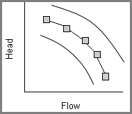
SWMM treats pumps as links that have a pre-defined relationship between flow rate Q and head H or some suitable surrogate. This relationship is defined by a user-supplied Pump Curve. Table 6-1 depicts the five types of pump curves that SWMM recognizes. Although not a requirement, a pump's inlet node would typically be a storage node that represents a pump station's wet well. An exception would be an inline booster pump placed inside a force main line under dynamic wave analysis. A sixth type of pump, called an Ideal pump, does not use a pump curve but instead has its flow rate equal the inflow rate into its inlet node. It must be the only outflow link from its inlet node and is used mainly for preliminary design.
A single point on a Type1 or Type2 curve would typically represent an operating point for a constant flow positive displacement pump. Additional points might represent flow rates at different pump speeds or contributions from additional constant speed pumps running in parallel. The Type3 curve represents the characteristic curve of a centrifugal pump operating at some fixed speed, where there is a continuous range of flows available depending on the head required. The Type4 curve could be a positive displacement pump with continuous speed control or a centrifugal pump that lifts water to a more or less fixed elevation so that the required head depends only on the water level at its inlet node. A Type5 pump is a variable speed version of the Type3 pump. As the pump's impeller speed varies relative to some nominal value, flow changes in direct proportion while head changes in proportion to speed squared.
Whenever a pump link is encountered in either the dynamic wave or kinematic wave methods its new flow is found directly from its pump curve using whatever values were last computed for nodal heads and volumes.
Table 6‑1 Pump curves recognized by SWMM
| Type | Description | Image |
|---|---|---|
| Type1 | Consists of a series of constant flow rates that apply over a corresponding series of volume intervals at the pump's inlet node. |
|
| Type2 | Similar to a Type1 pump except that the fixed flow rate levels vary over a set of depth intervals at the pump's inlet node. |
|
| Type3 | A centrifugal pump characteristic curve at some nominal impeller speed represented in a piecewise linear fashion. Flow is a function of the head difference between the inlet and outlet nodes. |
|
| Type4 | A variable speed in-line pump where flow varies continuously with inlet node depth. |
|
| Type5 | A variable speed version of the Type3 pump where the head v. flow curve shifts position depending on the pump's speed setting. |
|
For Type1 and Type 2 curves, the curve is searched in step-wise fashion for the first point whose volume or depth exceeds the volume or depth at the pump's inlet node. The pump's flow is the flow associated with that point. For the Type3 and Type5 curves, the flow is determined by first finding the pair of adjacent data points that bracket the difference in head between the pump's outlet and inlet nodes and then interpolating a flow between these points for the given head difference. A similar lookup procedure is used for the Type4 curve except that water level at the pump's inlet node is used instead of head difference. A pump's flow is not allowed to be outside the minimum and maximum values defined by its pump curve and is not allowed to be negative.
The Type5 pump curve is shifted depending on what relative speed setting ω the pump is currently operating under, where a setting of 1.0 applies to the original user-supplied curve. Following the pump affinity laws (Sanks et al., 1998), a point with head H and flow Q on the original curve becomes \(\omega^{2}H\) and \(\omega Q\), respectively on the speed-adjusted curve. For the other pump types only the flow value found from the original curve is multiplied by the speed setting.
Speed settings can be changed during a simulation by using control rules. The setting can also be used to control pump operation based on wet well level (e.g., set ω to 1 when the level is above a startup depth and to 0 when below a shutoff depth). The adjusted pump flow is checked to insure it does not cause the water level at the inlet node to drop below 0 over the current time step. If the node is a storage node then the pumping rate cannot exceed Qmax where
\[Q_{\max} = Q_{in} + \frac{V_{N}}{\Delta t}\]
(6-1)
and Qin is the most recently computed total inflow to the node, VN is the node volume at the start of the time step, and ∆t is the current time step interval. If the inlet node is not a storage node and dynamic wave analysis is being made, Equation 3-15a is used with the current pumping rate to estimate what the inlet node head at the end of the time step would be. If this head is below the node's invert elevation then the pumping rate is set equal to the node's current inflow.
Some additional computational details regarding pumps are as follows:
For dynamic wave modeling:
a. Pumps do not contribute any surface area to the node-link assemblies at their inlet and outlet nodes.
b. For Type3, Type4 and Type5 pump curves the \(\frac{\partial Q}{\partial H}\) term used for evaluating a surcharged node is the negative of the slope of the line segment on which the pumping rate lies. For the other pump types it is zero since their line segments have zero slope.
c. No under-relaxation is applied to consecutive pump flows at Step 3 of the iterative solution method described in Section 3.2.
SWMM computes the power consumed in kilowatt-hours by each pump over each time step ∆t as:
\[Kwh = 0.7457\left( H_{2} - H_{1} \right)\frac{Q\left( \frac{\Delta t}{3600} \right)}{8.814}\]
(6-2)
where heads H1 and H2 are in feet, flow Q is in cfs, and time step ∆t is in seconds. The pump's wire to water efficiency is not included in this calculation. The power consumption in each time period is totaled up and reported for each pump in SWMM's Pumping Summary Report. Also reported are the percent of time each pump is online and operates at either the lower or upper end of its pump curve.
Orifices are regularly shaped, submerged openings through which flow is proportional to the square root of the head across the opening. Orifices are typically used to:
SWMM represents an orifice as a link between two nodes. The opening can be oriented either in a vertical plane for a side orifice or in a horizontal plane for a bottom orifice (see Figure 6-1) and be elevated some distance above the inlet node's invert. A riser pipe or inlet box used as an outlet structure in a detention pond can be modeled as a bottom orifice with a vertical offset. For kinematic wave analysis the inlet node must be a storage node since this is the only type of node for which a true hydraulic head is computed. For dynamic wave analysis it can be any type of node.
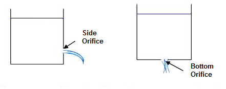
Figure 6‑1 Orifice orientations
The properties of an orifice link include:
The size of the orifice opening can be changed during a simulation by having its setting adjusted using control rules. An orifice's setting is the fraction of its full height that remains open (such as would occur due to the action of lowering or raising a sluice gate above a side orifice). In this case an additional optional parameter is the time it takes to fully close a completely open (or fully open a completely closed) orifice.
Whenever an orifice link is encountered in the dynamic wave or kinematic wave solution procedure with its inlet side fully submerged its flow rate Q (cfs) can be found using Torricelli's equation (Brater et al., 1996):
\[Q = C_{d}A_{O}\sqrt{2gH_{e}}\]
(6-3)
where Cd is a dimensionless orifice discharge coefficient, AO is the area of the opening (ft2), and He is the effective head seen by the orifice (ft). The following paragraphs describe how each of these parameters is evaluated.
Discharge Coefficient (Cd)
The most commonly cited value for Cd is 0.6 while 0.4 is recommended for ragged edge orifices (Federal Highway Administration, 2009). Brater et al. (1996) review a number of experimental studies that show the coefficient varying between 0.59 and 0.67 depending on orifice shape, size, and effective head.
Area of Opening (AO)
The area of the orifice's opening depends on what its setting is. Let ω be the orifice setting (between 0 and 1) in place at the end of the previous routing time step and ω* be the target setting that was established the last time that a control rule involving the orifice was activated. If the time to close/open the orifice, ∆t~O\ ~, is 0 then for the current time step ω = ω*. Otherwise let ∆ω be defined as ω* - ω and ω gets updated as follows:
| Condition | Value | Equation |
|---|---|---|
| if \(\frac{\Delta t}{{\Delta t}_{O}} < \Delta\omega\) | \(\omega + \frac{sgn(\Delta\omega)\Delta t}{{\Delta t}_{O}}\) | (6-4) |
| otherwise | \(\omega^{*}\) |
where ∆t is the length of the current time step. With the setting established, the area of the orifice opening is determined using the methods described in Chapter 5 to find the area of either a circular or rectangular cross section, depending on orifice shape, at a fraction ω of its full height.
Effective Head (He)
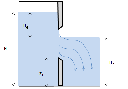
The effective head across the orifice depends on whether the water level on its outflow side is below the orifice opening or not. Let H1 be the most recently computed head at the orifice's nominal upstream node and H2 be the same at the nominal downstream node. For kinematic wave analysis, since the upstream node must be a storage node, H1 is the water surface elevation in the storage unit while H2 is the invert elevation of the downstream node. If \(H_{1} < H_{2}\) and the orifice does not have a flap gate then the head values are reversed (so H1 has the higher value) and the computed flow will be opposite to the nominal downstream direction.
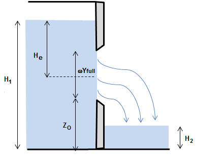
With H1 and H2 established the following rules are used to determine the effective head across the orifice, where ZO is the elevation of the bottom of the orifice opening and Yfull is its full height:
| Condition | Value | Equation |
|---|---|---|
| for \(H_{2} < Z_{O} + \omega\frac{Y_{full}}{2}\) | \(H_{1} - \left( Z_{O} + \omega\frac{Y_{full}}{2} \right)\) | (6-5) |
| otherwise | \(H_{1} - H_{2}\) |
| Condition | Value | Equation |
|---|---|---|
| for \(H_{2} \leq Z_{O}\) | \(H_{1} - Z_{O}\) | (6-6) |
| otherwise | \(H_{1} - H_{2}\) |
Figure 6-2 illustrates how He is evaluated for a side orifice.
When the water level at the inlet to a side orifice is below the top of its opening the orifice behaves more like a weir and Equation 6-3 no longer applies (see Figure 6-3). A similar situation occurs when the head above a bottom orifice is below some threshold level. For these cases SWMM determines what the threshold head for weir behavior is and what the equivalent weir coefficient and crest length should be when using the standard rectangular weir formula to compute the orifice's flow rate. The details differ for side and bottom orifices as described below.
Submerged Upstream Only Submerged Both Up and Downstream
Figure 6‑2 Determination of effective head for an orifice
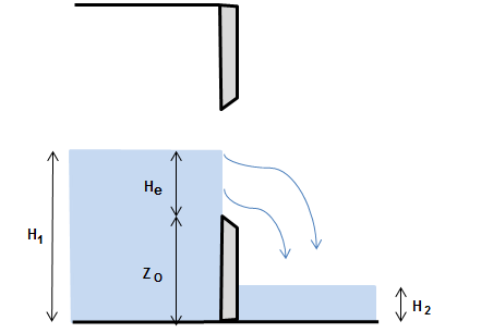
Figure 6‑3 Orifice with unsubmerged inlet
Side Orifices
For a side orifice, weir behavior occurs when the inlet water level is below the top of the orifice opening. Thus the threshold head H* is:
\[H^{*} = Z_{O} + \omega Y_{full}\]
(6-7)
When the inlet head H1 is below this height the flow through the orifice can be approximated by using the general weir formula:
\[Q = C_{W}L\left( H_{1} - Z_{O} \right)^{1.5}\]
(6-8)
where CW is a weir coefficient (ft1/2/sec) and L is the crest length of the equivalent weir (ft). Equating the flow from this equation to that from the orifice equation 6-3 when \(H_{1} = H^{*}\) and solving for CWL results in:
\[C_{W}L = \frac{C_{d}A_{O}\sqrt{g}}{\omega Y_{full}}\]
(6-9)
Thus whenever the upstream head H1 is below H**, flow through the side orifice can be found using the weir formula 6-8 with CWL given by Equation 6-9.
Bottom Orifices
For a bottom orifice it is assumed that the threshold inlet head H* for weir flow will be at a point where the flow through the orifice using both the orifice and general weir equations will be the same. In equation terms:
\[C_{d}A_{O}\sqrt{2g}\left( H^{*} - Z_{O} \right)^{0.5} = C_{W}L\left( H^{*} - Z_{O} \right)^{1.5}\]
(6-10)
Solving for H* results in:
\[H^{*} = Z_{O} + \frac{C_{d}A_{O}\sqrt{2g}}{C_{W}L}\]
(6-11)
In order to evaluate H** values for CW and L must be assigned. CW can be set to the commonly cited value of 3.33 ft0.5/sec used for sharp crested weirs (Mays, 2001). L can be set to the circumference of the opening as follows:
| Opening Type | Value | Equation |
|---|---|---|
| for a circular opening | \(\pi\omega Y_{full}\) | (6-12) |
| for a rectangular opening | \(2\left( b + \omega Y_{full} \right)\) |
where b is the fixed width of the rectangular opening. Now H** can be determined for a given orifice coefficient and opening dimensions. Whenever the upstream head H1 is below H**, flow through the bottom orifice can be found using the general weir formula 6-8 with CW = 3.33 and L given by Equation 6-12.
Tailwater Submergence Correction
As described later on in Section 6.3, whenever the downstream water level is above a weir's crest the Villemonte equation is applied to account for the effects of submergence (Brater et al., 1996). So when the general weir equation 6-8 is used to compute orifice flow and the downstream head H2 is above the bottom of the orifice opening ZO, the following submergence adjustment factor fS is applied to the computed flow value:
\[f_{S} = \left\lbrack 1 - \left( \frac{H_{2}}{H_{1}} \right)^{1.5} \right\rbrack^{0.385}\]
(6-13)
When an orifice has a flap gate it adds a small amount of head loss for flow through the gate. An empirical formula for this head loss was derived from experiments performed at Iowa State University in the 1930's and published by Armco (1978):
\[\Delta H = \frac{4U^{2}}{g}\exp\left( - 1.15\frac{U}{\sqrt{H_{e}}} \right)\]
(6-14)
where ∆H is the head loss added by the flap gate (ft) and U is the velocity through the orifice (ft/sec) which equals \(\frac{Q}{A_{O}}\). After the orifice's flow is first computed without this additional head loss, ∆H is computed with Equation 6-14 and subtracted from He. Then the flow is re-computed, this time using the adjusted value of effective head.
Dynamic wave modeling uses the surface area of the links attached to a node to update the node's head when it is not in a surcharged state (see Chapter 3). As an orifice has no length, its contribution to a node's surface area should be zero. However in older versions of SWMM an orifice was represented as an equivalent pipe that contributed surface area to its end nodes just as a real conduit did. To maintain compatibility with previous versions, SWMM 5 computes a surface area ASL for an orifice as
| Orifice Type | Value | Equation |
|---|---|---|
| for a side orifice | \(W(Y_{O})L_{O}\) | (6-15) |
| for a bottom orifice | \(A\left( \omega Y_{full} \right)\) |
where:
YO = depth of flow through the orifice (ft), equal to \(\min\left( H_{1} - Z_{O}\ ,\ \omega Y_{full} \right)\)
LO = equivalent conduit length of the orifice (ft), equal to
\[\max\left( 2{\Delta t}_{\max}\sqrt{gY_{full}}\ ,200 \right)\]
∆tmax = maximum time step assigned by the user to the simulation (sec)
W(Y) = width of orifice opening at flow depth Y (ft)
A(Y) = area of orifice opening at flow depth Y (ft)
W(Y) and A(Y) are evaluated using the formulas from Chapter 5 for either a circular or closed rectangular cross section shape. Half of ASL is assigned to each of the orifice's end nodes providing that the node is not a storage unit nor has its head below the orifice opening.
Dynamic wave analysis also needs a value for the derivative of a link's flow rate with respect to head (dQ/dH) when updating the head for a surcharged node connected to the link (see section 3.3.5). For submerged headwater orifices that use Equation 6-3 to compute flow rate Q, this derivative is:
\[\frac{dQ}{dH} = 0.5\frac{Q}{H_{e}}\]
(6-16)
while for unsubmerged headwater orifices that use Equation 6-8 to compute Q it is:
\[\frac{dQ}{dH} = 1.5\frac{Q}{\left( H_{1} - Z_{O} \right)}\]
(6-17)
The computational steps used to compute flow through an orifice link can be summarized as follows. At the start of a time step:
For each iteration within a time step that requires computing flow through the orifice:
A transverse weir is a barrier with a cut-out placed across a conduit perpendicular to the direction of flow. A side weir is a cut-out along the side wall of a conduit parallel to the direction of flow. Flow through a weir is proportional to the height of water above the weir's crest raised to a power greater than one. Weirs are used for the same types of reasons as orifices: to regulate flow out of storage facilities, to regulate flow through channels, and to divert excess flow from interceptor sewers to overflow structures. While orifices normally operate with their inlet sides submerged, weirs normally maintain a free surface above them.
SWMM represents a weir as a link between two nodes. For kinematic wave analysis the inlet node must be a storage node since this is the only type of node for which a true hydraulic head is computed. For dynamic wave analysis it can be any type of node.
The properties of a weir link include:
Figure 6-4 shows the different shapes of transverse weirs modeled by SWMM. The only shape allowed for a side weir is rectangular.
Figure 6‑4 Transverse weir shapes
A suppressed rectangular weir has its opening extended across the entire channel while a contracted weir does not. Weirs are also classified as being sharp-crested or broad-crested. Sharp-crested weirs have a relatively short crest thickness so that water springs clear of the crest as it flows over the weir. The crest of a broad-crested weir is thick enough so that the overflow remains in contact with the crest surface.
The elevation of a weir's crest can be changed during a simulation by having its setting adjusted using control rules. A weir's setting ω is the fraction of its full height that remains open after it's crest is moved up or down, as might occur with a downward opening weir gate or inflatable dam. At a setting of 1 the weir's crest position is at its lowest possible value and the full height of its opening is available for flow. At a value of 0 the crest has been raised so that no opening height remains and no flow can pass through the weir. At intermediate settings the crest elevation equals its lowest possible value plus 1 - ω times its full opening height.
General Equations
The general equation for free flow over a transverse rectangular weir is (Brater et al., 1996):
\[Q = C_{W}L_{e}H_{e}^{3/2}\]
(6-18)
and for a triangular weir is (Brater et al., 1996):
\[Q = C_{W}\tan\left( \frac{\theta}{2} \right)H_{e}^{5/2}\]
(6-19)
In these equations Q is the flow rate (cfs), Le is the effective crest length (ft), θ is the slot angle of a triangular weir, He is the effective head seen by the inflow side of the weir (ft), and CW* is a weir coefficient (ft1/2/sec). A trapezoidal weir can be treated as a combination of a rectangular weir and two half-triangular weirs (Featherstone and Nalluri, 1982) leading to the equations:
\[Q = Q_{R} + Q_{T}\]
(6-20a)
\[Q_{R} = C_{WR}L_{e}H_{e}^{3/2}\]
(6-20b)
\[Q_{T} = C_{WT}sH_{e}^{5/2}\]
(6-20c)
where s is the slope (run / rise) of the trapezoidal side wall and CWR and CWT are the coefficients that apply to the rectangular and triangular portions of the weir, respectively.
Effective Head (He)
The effective head seen by a weir, accounting for its current setting, is:
\[H_{e} = H_{1} - \left( Z_{W} + (1 - \omega)Y_{full} \right)\]
(6-21)
where H1 is the higher of the heads at the weir's end nodes, ZW* is the elevation of the weir's crest when fully open (i.e., when ω = 1), and Yfull is the full height of the weir's opening. If H1* corresponds to the downstream node of the weir then reverse flow occurs through the weir unless a flap gate is present in which case the flow is
Effective Crest Length (Le)
The effective crest length of a rectangular weir is reduced by the number of end contractions as follows (Mays, 2001):
\[L_{e} = L - 0.1nH_{e}\]
(6-22)
where L is the actual crest length and n = 1 if the weir is placed away from one side wall, n = 2 if it is placed away from both side walls and n = 0 if it occupies the entire width of the conduit (see Figure 6-4).
When the setting ω for a triangular weir is less than 1 its opening takes the shape of a trapezoidal weir. In this case the trapezoidal weir equation 6-18 is used with both CWR and CWT set equal to the weir's original coefficient, the side wall slope s set equal to \(\tan\left( \frac{\theta}{2} \right)\) and the effective length becomes:
\[L_{e} = 2s(1 - \omega)Y_{full}\]
(6-23)
This equation is also used for a trapezoidal weir whose setting is less than 1.
Weir Coefficient (CW)
The standard weir coefficient CW for a sharp crested rectangular weir is 3.33 ft1/2/sec (Mays, 2001). For \(\frac{H_{W}}{L} > \frac{1}{3}\) the coefficient has been found to vary with effective head and weir sizing and placement (Bureau of Reclamation, 2001). The Kindsvater-Carter method (Bureau of Reclamation, 2001) expresses this dependence with the following formula:
\[C_{W} = c1\left( \frac{H_{W}}{Z_{W}} \right) + c2\]
(6-24)
where the constants c1 and c2 vary with the ratio of the crest length L to the full width b of the cross section in which the weir is placed as listed in Table 6-2.
Broad crested weir behavior is considered to occur when the ratio of the water level above the crest to the crest thickness exceeds a certain limit. Limits of 1 to 2 have been proposed by Brater et al. (1996), 15 by French (1985), and 2 to 20 by the Bureau of Reclamation (2001). Table 6-3 is a compilation of broad-crested weir coefficients synthesized by Brater and King (1976) from several different experimental studies. It shows the dependence of the coefficient on both head and breadth of crest. Above a ratio of about 2 the weir behaves as sharp-crested with a coefficient of 3.32. For ratios below 0.5 the coefficient approaches 2.63.
Table 6‑2 Kindsvater-Carter constants for rectangular weir coefficient
| L/b | **c1 (ft1/2/sec)** | **c2 (ft1/2/sec)** |
|---|---|---|
| 0.2 | -0.0087 | 3.152 |
| 0.4 | 0.0317 | 3.164 |
| 0.5 | 0.0612 | 3.173 |
| 0.6 | 0.0995 | 3.178 |
| 0.7 | 0.1602 | 3.182 |
| 0.8 | 0.2376 | 3.189 |
| 0.9 | 0.3447 | 3.205 |
| 1.0 | 0.4000 | 3.220 |
The standard value for the triangular weir coefficient CW is 2.5 ft1/2/sec (Mays, 2001). Figure 6-5 shows the variation of CW (in ft1/2/sec ) with head over the weir HW (in feet) presented by Brater and King (1976). The range of coefficients is rather small, from 2.5 up to 2.8.
Figure 6‑5 Coefficient for triangular weirs (from Brater and King, 1976)
**Table 6‑3 Rectangular broad-crested weir coefficients (ft1/2/sec)**
| Head (ft) | 0.5 | 0.75 | 1.00 | 1.5 | 2.0 | 2.5 | 3.00 | 4.00 | 5.00 | 10.00 | 15.00 |
|---|---|---|---|---|---|---|---|---|---|---|---|
| 0.2 | 2.80 | 2.75 | 2.69 | 2.62 | 2.54 | 2.48 | 2.44 | 2.38 | 2.34 | 2.49 | 2.68 |
| 0.4 | 2.92 | 2.80 | 2.72 | 2.64 | 2.61 | 2.60 | 2.58 | 2.54 | 2.50 | 2.56 | 2.70 |
| 0.6 | 3.08 | 2.89 | 2.75 | 2.64 | 2.61 | 2.60 | 2.68 | 2.69 | 2.70 | 2.70 | 2.70 |
| 0.8 | 3.30 | 3.04 | 2.85 | 2.68 | 2.60 | 2.60 | 2.67 | 2.68 | 2.68 | 2.69 | 2.64 |
| 1.0 | 3.32 | 3.14 | 2.98 | 2.75 | 2.66 | 2.64 | 2.65 | 2.67 | 2.68 | 2.68 | 2.63 |
| 1.2 | 3.32 | 3.20 | 3.08 | 2.86 | 2.70 | 2.65 | 2.64 | 2.67 | 2.66 | 2.69 | 2.64 |
| 1.4 | 3.32 | 3.26 | 3.20 | 2.92 | 2.77 | 2.68 | 2.64 | 2.65 | 2.65 | 2.67 | 2.64 |
| 1.6 | 3.32 | 3.29 | 3.28 | 3.07 | 2.89 | 2.75 | 2.68 | 2.66 | 2.65 | 2.64 | 2.63 |
| 1.8 | 3.32 | 3.31 | 3.31 | 3.07 | 2.88 | 2.74 | 2.68 | 2.66 | 2.65 | 2.64 | 2.63 |
| 2.0 | 3.32 | 3.30 | 3.30 | 3.03 | 2.85 | 2.76 | 2.72 | 2.68 | 2.65 | 2.64 | 2.63 |
| 2.5 | 3.32 | 3.31 | 3.31 | 3.28 | 3.07 | 2.89 | 2.81 | 2.72 | 2.67 | 2.64 | 2.63 |
| 3.0 | 3.32 | 3.32 | 3.32 | 3.32 | 3.20 | 3.05 | 2.92 | 2.73 | 2.66 | 2.64 | 2.63 |
| 3.5 | 3.32 | 3.32 | 3.32 | 3.32 | 3.32 | 3.19 | 2.97 | 2.76 | 2.68 | 2.64 | 2.63 |
| 4.0 | 3.32 | 3.32 | 3.32 | 3.32 | 3.32 | 3.32 | 3.07 | 2.79 | 2.70 | 2.64 | 2.63 |
| 4.5 | 3.32 | 3.32 | 3.32 | 3.32 | 3.32 | 3.32 | 3.32 | 2.88 | 2.74 | 2.64 | 2.63 |
| 5.0 | 3.32 | 3.32 | 3.32 | 3.32 | 3.32 | 3.32 | 3.32 | 3.07 | 2.79 | 2.64 | 2.63 |
| 5.5 | 3.32 | 3.32 | 3.32 | 3.32 | 3.32 | 3.32 | 3.32 | 3.32 | 2.88 | 2.64 | 2.63 |
Flow through a rectangular side weir is a case of spatially varied flow with decreasing discharge and varying flow depth with distance along the weir. Mays (2001) cites a number of different studies that have developed discharge equations for side weirs where both the head and weir coefficient vary spatially. Unfortunately these approaches are too complex to implement in a program like SWMM. The empirical Engels equation (Metcalf & Eddy, Inc. 1972) is used instead:
\[Q = C_{W}L_{e}^{0.83}H_{e}^{1.67}\]
(6-25)
Where flow Q is in cfs, length Le and head He are in feet, and CW is in ft1/2/sec. (It should be noted that previous versions of SWMM used an incorrect form of this equation that had the exponent on Le equal to 1.0)
Equation 6-25 applies to positive flow through the weir. For reverse flow the standard rectangular weir equation 6-18 is used. CW was assigned a value of 3.32 in the original Engels equation. Brunner (2014) notes that side weir coefficients should be lower than the typical values used for transverse weirs, and suggests a range of 1.5 to 2.6 for weirs that model levees or roadways along natural channels.
As shown in Figure 6-6, submerged weir flow occurs when the water level on the downstream side of the weir (H2) is above the crest elevation (ZW). Under this condition weir flow is related not only to the head on the upstream side of the weir (H1) but also to H2 and ZW* (Brater et al., 1996). These effects are commonly accounted for by applying an adjustment factor fS developed by Villemonte (1947) to the flow computed using the free flow equation:
\[f_{S} = \left\lbrack 1 - \left( \frac{H_{2}}{H_{1}} \right)^{n} \right\rbrack^{0.385}\]
(6-26)
where n is the exponent on head used in the weir flow equation and the heads H1 and H2 are in feet. For transverse rectangular weirs (Equation 6-18) it is 3/2, for side weirs (Equation 6-25) it is 1.67, and for triangular weirs (Equation 6-19) it is 5/2. For trapezoidal weirs separate submergence factors are computed for the rectangular flow portion (QR in Equation 6-20b with n = 3/2) and for the triangular flow portion (QT in Equation 6-20c with n = 5/2).
Figure 6‑6 Definitions of submerged and surcharged weir flow
As shown in Figure 6-4, the weirs modeled by SWMM assume that the top of the flow opening extends to the top of the structure that houses the weir. If this structure is an open channel then the highest head that the weir can see is \({\omega Y}_{full}\) where ω reflects the weir's current setting. If the structure encloses the weir from above, such as in a sewer pipe, then the head on the upstream side of the weir can exceed the structure's crown elevation causing the weir to become surcharged (see Figure 6-6). In this case the weir acts as an orifice and its flow should be evaluated using the equivalent of Equation 6-3:
\[Q = C_{d}A_{O}\sqrt{2gH_{e}} = C_{O}\sqrt{H_{e}}\]
(6-27)
where CO is an equivalent orifice constant with units of ft5/2/sec.
CO can be evaluated by setting Equation 6-27 equal to the appropriate weir equation (6-18, 6-19, 6-20, or 6-25 depending on weir type) evaluated at a weir head
\[H_{e} = {\omega Y}_{full}\]
for which the corresponding orifice head would be
\[\frac{{\omega Y}_{full}}{2}\]
. The result is:
\[C_{O} = \frac{Q_{W}\left( {\omega Y}_{full} \right)}{\sqrt{\frac{{\omega Y}_{full}}{2}}}\]
(6-28)
where
\[Q_{W}\left( {\omega Y}_{full} \right)\]
is the flow in cfs from the relevant weir equation for a head of \({\omega Y}_{full}\) feet. The constant CO is re-evaluated each time a weir's setting changes.
Thus if the user indicates that a weir is allowed to surcharge, then whenever the upstream head H1 is above ZW + Yfull its flow is computed using Equation 6-27. The head He to be used in this equation is computed as follows. Let H* be the head corresponding to the elevation at half of the weir's opening height, i.e.:
\[H^{*} = Z_{W} + (1 - \omega)Y_{full} + \frac{\omega Y_{full}}{2}\]
(6-29)
Then
| Condition | Value | Equation |
|---|---|---|
| for \(H_{2} < H^{*}\) | \(H_{1} - H^{*}\) | (6-30) |
| otherwise | \(H_{1} - H_{2}\) |
In addition, the correction for weir submergence is not applied.
When a weir has a flap gate it adds a small amount of head loss for flow through the gate. The same Armco formula used for orifices is used to compute this head loss for weirs:
\[\Delta H = \frac{4U^{2}}{g}\exp\left( - 1.15\frac{U}{\sqrt{H_{e}}} \right)\]
(6-31)
where ∆H is the head loss added by the flap gate (ft) and U is the velocity through the weir (ft/sec). To evaluate the velocity term in this equation one needs to know the effective area Ae of flow over the weir. This area equals
| Condition | Value | Equation |
|---|---|---|
| for normal weir flow | \(A\left( H_{W} + y_{C} \right) - A\left( y_{C} \right)\) | (6-32) |
| for surcharged weir flow | \(A\left( Y_{full} \right) - A\left( y_{C} \right)\) |
where Yfull is the full height of the weir opening, yC is the distance that the weir crest has been raised due to the current setting (equal to \((1 - \omega)Y_{full}\) ), and A(y) is the area of the weir opening at flow depth y. The latter quantity is found using the geometry functions described in Chapter 5 for either a rectangular, triangular, or trapezoidal shape. Knowing Ae, \(U = \frac{Q}{A_{e}}\), where the flow Q has been determined using the methods described in the previous sections.
After the orifice's flow is first computed without this additional head loss, ∆H is computed with Equation 6-31 and subtracted from He. Then the flow is re-computed, this time using the adjusted value of effective head.
A weir does not contribute any surface area to its end nodes under dynamic wave modeling. The derivative of its flow rate with respect to head (dQ/dH), used when updating the head of a surcharged end node (see section 3.3.5), is computed using the formulas in Table 6-4.
Table 6‑4 Formulas for flow derivatives of various types of weirs
| Weir Type | **Flow Derivative *(dQ/dH)*** |
|---|---|
| Transverse Rectangular | \(1.5\frac{\vert Q \vert}{H_{e}}\) |
| Side Flow Rectangular: | |
| a. \(Q \geq 0\) | \(1.67\frac{\vert Q \vert}{H_{e}}\) |
| b. \(Q < 0\) | \(1.5\frac{\vert Q \vert}{H_{e}}\) |
| Transverse Triangular: | |
| a. Fully open (ω = 1) | \(2.5\frac{\vert Q \vert}{H_{e}}\) |
| b. Partly open (ω < 1) | \(1.5\frac{\vert Q_{R} \vert}{H_{e}} + 2.5\frac{\vert Q_{T} \vert}{H_{e}}\) |
| Transverse Trapezoidal | \(1.5\frac{\vert Q_{R} \vert}{H_{e}} + 2.5\frac{\vert Q_{T} \vert}{H_{e}}\) |
Note: For trapezoidal openings, QR is the flow through the central rectangular portion and QT is the flow through the triangular end portions (see Equation 6-20).
The computational steps used to compute flow through a weir link can be summarized as follows. If the weir is allowed to surcharge and its setting ω changes at the start of a time step then use Equation 6-28 to compute an equivalent orifice coefficient CO to use during surcharge conditions. For each iteration within a time step that requires computing flow through the weir:
SWMM's outlet link is a generic type of flow regulator with a user defined rating curve that relates flow rate to effective head. It can be used in cases where the head-flow relationships that SWMM uses for orifice or weir links do not apply. Some examples would be:
For kinematic wave analysis the outlet's upstream node must be a storage node since this is the only type of node for which a true hydraulic head is computed. For dynamic wave analysis it can be any type of node.
The properties of an outlet link include:
An outlet link can also have a flow setting between 0 and 1 that can be modified by control rules. The setting serves as a multiplier applied to the flow determined from the outlet's rating curve.
The rating curve can be defined either as an analytical power law function or a tabular listing of points on the curve. The analytical power function has the form:
\[Q = aH_{e}^{b}\]
(6-33)
where Q is flow rate (cfs), He is the effective head (ft), and a and b are user-supplied constants. The tabular rating curve consists of pairs of head (He) and flow (Q) values for points that the user chooses to represent the shape of the outlet's rating curve.
Figure 6‑7 Rating curve for a vortex device compared to an orifice
The following steps are used whenever the flow through an outlet link must be computed:
 1.13.2