The movement of water through a conveyance network of channels and pipes is governed by the conservation of mass and momentum equations for gradually varied, unsteady free surface flow. Dynamic wave analysis solves the complete form of these equations and therefore produces the most theoretically accurate results. It can account for channel storage, backwater effects, entrance/exit losses, flow reversal, and pressurized flow. Because it couples together the solution for both water levels at nodes and flow in conduits it can be applied to any general network layout, even those containing multiple downstream diversions and loops. It is the method of choice for systems subjected to significant backwater due to downstream flow restrictions and with flow regulation via weirs and orifices. This generality comes at a price of having to use small time steps to maintain numerical stability.

Dynamic wave modeling was first introduced into version 3 of SWMM in 1981 as a separate program module known as EXTRAN (Extended Transport) (Roesner et al., 1983). The node-link solution method it uses had its origins in the Sacramento-San Joaquin Delta Model (Shubinski et al., 1965) and the WRE Transport Model (Kibler et al., 1975). Although more powerful solution techniques are available (such as implicit finite difference schemes (Cunge et al., 1980) and shock-capturing finite volume schemes (Toro, 2001)), SWMM 5 continues to use EXTRAN's node-link approach, with modifications made to enhance its stability, because of its simplicity and versatility.

3.1 Governing Equations

The conservation of mass and momentum for unsteady free surface flow through a channel or pipe are known as the St. Venant equations and can be expressed as:


\[\frac{\partial A}{\partial t} + \frac{\partial Q}{\partial x} = 0\]	Continuity	(3-1)
\[\frac{\partial Q}{\partial t} + \frac{\partial\left( \frac{Q^{2}}{A} \right)}{\partial x} + gA\frac{\partial H}{\partial x} + gAS_{f} = 0\]	Momentum	(3-2)

where


x	=	distance (ft)
t	=	time (sec)
A	=	flow cross-sectional area (ft²)
Q	=	flow rate (cfs)
H	=	hydraulic head of water in the conduit (Z + Y) (ft)
Z	=	conduit invert elevation (ft)
Y	=	conduit water depth (ft)
S_f	=	friction slope (head loss per unit length)
g	=	acceleration of gravity (ft/sec²)

The derivation of these equations can be found in standard texts such as Henderson (1966), Cunge et al. (1980) and French (1985). The assumptions on which they are based are:

flow is one dimensional
pressure is hydrostatic
the cosine of the channel bed slope angle is close to unity
boundary friction can be represented in the same manner as for steady flow.

The friction slope S_f can be expressed in terms of the Manning equation used to model steady uniform flow:

\[S_{f} = \left( \frac{n}{1.486} \right)^{2}\frac{Q|U|}{AR^{4/3}}\]

(3-3)

where


n	=	the Manning roughness coefficient (sec/m^1/3)
R	=	the hydraulic radius of the flow cross-section (ft)
U	=	flow velocity, equal to \(\frac{Q}{A}\) (ft/sec).

and 1.486 converts from m^1/3 to ft^1/3. Use of the absolute value sign on the velocity term makes S_f a directional quantity (since Q can be either positive or negative) and ensures that the frictional force always opposes the flow. Manning roughness coefficients for wide range of channel surfaces and pipe materials can be found in Appendix G.

For a specific cross-sectional geometry, the flow area A is a known function of water depth Y which in turn can be obtained from the head H. Thus the dependent variables in these equations are flow rate Q and head H, which are functions of distance x and time t. To solve these equations over a single conduit of length L, one needs a set of initial conditions for H and Q at time 0 as well as boundary conditions at x = 0 and x = L for all times t.

The continuity equation 3-1 can be combined with the momentum equation 3-2 to produce the following form of the momentum equation for a conduit (see sidebar below for details):

\[\frac{\partial Q}{\partial t} = 2U\frac{\partial A}{\partial t} + U^{2}\frac{\partial A}{\partial x} - gA\frac{\partial H}{\partial x} - gAS_{f}\]

(3-4)

Combining the Continuity and Momentum Equations

The \(\frac{\partial\left( \frac{Q^{2}}{A} \right)}{\partial x}\) term in the momentum equation 3-2 can be re-expressed as:

\[\frac{\partial\left( \frac{Q^{2}}{A} \right)}{\partial x} = \frac{\partial\left( U^{2}A \right)}{\partial x} = 2AU\frac{\partial U}{\partial x} + U^{2}\frac{\partial A}{\partial x}\]

(a)

Using \(Q = UA\), the continuity equation 3-1 can be written as:

\[\frac{\partial A}{\partial t} + A\frac{\partial U}{\partial x} + U\frac{\partial A}{\partial x} = 0\]

(b)

Multiplying both sides of (b) by \(U\) and re-arranging terms leads to:

\[AU\frac{\partial U}{\partial x} = - U\frac{\partial A}{\partial t} - U^{2}\frac{\partial A}{\partial x}\]

(c)

Substituting this into the first term on the right hand side of (a) produces:

\[\frac{\partial\left( \frac{Q^{2}}{A} \right)}{\partial x} = - 2U\frac{\partial A}{\partial t} - U^{2}\frac{\partial A}{\partial x}\]

(d)

Substituting (d) into 3-2 and re-arranging terms gives the final result:

\[\frac{\partial Q}{\partial t} = 2U\frac{\partial A}{\partial t} + U^{2}\frac{\partial A}{\partial x} - gA\frac{\partial H}{\partial x} - gAS_{f}\]

(e)

While this equation can be used to compute the time trajectory of flow in a conduit, another relationship is needed to do likewise for heads. SWMM's node – link representation of the conveyance network, conceptualized in Figure 3-1, does this by providing a continuity relationship at junction nodes that connect conduits together within a conveyance network. As shown in the figure, a continuous water surface is assumed to exist between the water elevation at a node and in the conduits that enter and leave it. Two types of nodes are possible. Non-storage junction nodes are assumed to be points with zero volume and surface area while storage nodes (such as ponds and tanks) contain both volume and surface area.

Node-Link.bmp

Figure 3-1 Node-link representation of a conveyance network in SWMM (from Roesner et al, 1992).

Each "node assembly" consists of the node itself and half the length of each link connected to it. Conservation of flow for the assembly requires that the change in volume with respect to time equal the difference between inflow and outflow. In equation terms:

\[\frac{\partial V}{\partial t} = \frac{\partial V}{\partial H}\frac{\partial H}{\partial t} = A_{S}\frac{\partial H}{\partial t} = \sum_{}^{}Q\]

(3-5)

where:


V	=	node assembly volume (ft³)
A_S	=	node assembly surface area (ft²)
ΣQ	=	net flow into the node assembly (inflow – outflow) (cfs)

The \(\sum_{}^{}Q\) term includes the flow in the conduits connected to the node as well as any externally imposed inflows such as wet weather runoff or dry weather sanitary flow.

Each node assembly's surface area consists of the node's storage surface area A_SN (if it's a storage node) plus the surface area contributed by the links connected to it, \(\sum_{}^{}A_{SL}\), where A_SL is the surface area contributed by a connecting link. Thus the node continuity equation can be written as:

\[\frac{\partial H}{\partial t} = \frac{\sum_{}^{}Q}{A_{SN} + \sum_{}^{}A_{SL}}\]

(3-6)

The flow depth at the end of a conduit connected to a node can be computed as the difference between the head at the node and the invert elevation of the conduit. The node and link surface areas are computed as functions of their respective flow depths.

Equations 3-4 and 3-6 provide a coupled set of partial differential equations that solve for flow Q in the conduits and head H at the nodes of the conveyance network. Because they cannot be solved analytically a numerical solution procedure must be used instead.

3.2 Solution Method

The material that follows applies to networks containing only conduits. Inclusion of flow control devices (pumps, orifices, and weirs) and other processes (seepage, evaporation, and minor losses) will be covered in subsequent chapters of this manual.

The spatial and temporal derivatives in equations 3-4 and 3-6 can be replaced with the following finite difference approximations:

\[\frac{\partial A}{\partial x} = \frac{\left( A_{2} - A_{1} \right)}{L}\]

(3-7)

\[\frac{\partial H}{\partial x} = \frac{\left( H_{2} - H_{1} \right)}{L}\]

(3-8)

\[\frac{\partial A}{\partial t} = \frac{\mathrm{\Delta}\overline{A}}{\mathrm{\Delta}t}\]

(3-9)

\[\frac{\partial Q}{\partial t} = \frac{\mathrm{\Delta}Q}{\mathrm{\Delta}t}\]

(3-10)

\[\frac{\partial H}{\partial t} = \frac{\mathrm{\Delta}H}{\mathrm{\Delta}t}\]

(3-11)

where


A₁	=	flow area at the upstream end of the conduit (ft²)
A₂	=	flow area at the downstream end of the conduit (ft²)
H₁	=	hydraulic head at the upstream end of the conduit (ft)
H₂	=	hydraulic head at the downstream end of the conduit (ft)
L	=	conduit length (ft)
∆t	=	time step (sec)
∆ \(\ \overline{A}\)	=	change in average flow area, \(\left( {\overline{A}}^{t + \mathrm{\Delta}t} - {\overline{A}}^{\ t} \right)\), over time step ∆t (ft²)
∆Q	=	change in conduit flow, \(\left( Q^{t + \mathrm{\Delta}t} - Q^{t} \right)\), over time step ∆t (cfs)
∆H	=	change in nodal head, \(\left( H^{t + \mathrm{\Delta}t} - H^{t} \right)\), over time step ∆t (ft).

with the superscripts referring to time periods.

Substituting these finite difference approximations into the link momentum Equation 3-4, replacing S_f with Equation 3-3, and replacing A, U, and R with their average values over the conduit length (as indicated by over scores) allows the finite difference form of the link momentum equation to be written as:

\[\frac{\mathrm{\Delta}Q}{\mathrm{\Delta}t} = 2\overline{U}\frac{\mathrm{\Delta}\overline{A}}{\mathrm{\Delta}t} + {\overline{U}}^{2}\frac{\left( A_{2} - A_{1} \right)}{L} - g\overline{A}\frac{\left( H_{2} - H_{1} \right)}{L} - g\eta^{2}\frac{Q\left| \overline{U} \right|}{{\overline{R}}^{4/3}}\]

(3-12)

where \(\eta = \frac{n}{1.486}\). Average values for A, U, and R can be approximated using the heads H₁ and H₂ as described later on in section 3.3.1.

The finite difference form of the nodal continuity equation 3-6 is:

\[\frac{\Delta H}{\Delta t} = \frac{\sum Q}{A_{SN} + \sum A_{SL}}\]

(3-13)

Previous versions of SWMM used an explicit forward Euler method (or more precisely the two-step Modified Euler method) to solve Equation 3-12, where known values of Q, H, A, \(\overline{A}\), \(\overline{U}\), and \(\overline{R}\) at time t were used to solve for Q at time t + ∆t. Then Equation 3-13 was solved with the new conduit flows to find new head values H at time t + ∆t.

SWMM 5 uses an implicit backwards Euler method instead to provide improved stability (Ascher and Petzold, 1998). Under this scheme Equation 3-12 is re-written as:

\[Q^{t + \Delta t} = \frac{Q^{t} + \Delta Q_{inertia} + \Delta Q_{pressure}}{1 + \Delta Q_{friction}}\]

(3-14)

where the terms are defined as:

Inertial Term (3-14a):
\[\Delta Q_{inertia} = 2\overline{U}( \overline{A}^{t + \Delta t} - \overline{A}^{t} ) + \overline{U}^{2}\frac{( A_{2} - A_{1} )}{L}\Delta t\]
Pressure Term (3-14b):
\[\Delta Q_{pressure} = - g\overline{A}\frac{( H_{2} - H_{1} )}{L}\Delta t\]
Friction Term (3-14c):
\[\Delta Q_{friction} = g\eta^{2}\frac{\lvert \overline{U} \rvert\Delta t}{\overline{R}^{4/3}}\]

and now H and the quantities A, \(\overline{A}\), \(\overline{U}\), and \(\overline{R}\) derived from it are all evaluated at the new time t+∆t. The finite difference form of the nodal continuity equation 3-12 can be expressed as:

\[H^{t + \mathrm{\Delta}t} = H^{t} + \frac{\frac{\Delta t}{2}\left( \sum_{}^{}{Q^{t} + \sum_{}^{}Q^{t + \mathrm{\Delta}t}} \right)}{\left( A_{SN} + \sum_{}^{}A_{SL} \right)^{t + \mathrm{\Delta}t}}\]

for non-outfall (3-15a)

\[H^{t + \mathrm{\Delta}t} = H_{Outfall}\]

for outfall nodes (3-15b)

H_Outfall is a user-supplied value that sets the head at a terminal outfall node. It can be a constant value, a value extracted from a user-supplied time series, or the elevation of the critical or normal flow depth in the connecting conduit. For the latter option, critical or normal depth is computed internally as a function of the conduit's flow rate and geometry as described in Chapter 5.

Equations 3-14 and 3-15 can be solved implicitly over a given time step ∆t using functional iteration (also known as successive approximations or Picard's method). The method is described in the sidebar titled "*Dynamic Wave Solution Procedure*". Because flows and heads are updated one conduit and node at a time and not simultaneously, the results at each time step are invariant to the order in which the conduits and links are evaluated. This allows Steps 2 and 4 of the solution procedure to be implemented using separate threads running in parallel on multi-processor computers which can offer a significant reduction in computation time.

3.3 Computational Details

3.3.1 Average Cross-Section Properties

Evaluation of the flow updating formula 3-14 requires values for the average area ( \(\overline{A}\)), hydraulic radius ( \(\overline{R}\)), and velocity ( \(\overline{U}\)) for the conduit in question. These values are computed using heads H₁ and H₂ belonging to the most recently computed head estimates *H^last* at either end of the conduit. The flow depth Y₁ at the upstream end of the conduit is computed as:

\[0 \text{ for } H_{1} \leq Z_{1}\]

\[H_{1} - Z_{1} \text{ for } Z_{1} < H_{1} \leq Z_{1} + Y_{full}\]

\[Y_{full} \text{ for } H_{1} > Z_{1} + Y_{full}\]

(3-16)

where Z*₁* is the elevation of the invert of the upstream end of the conduit and Y_full is the full depth of the conduit. A similar expression using H₂ and Z₂ applies to Y₂ at the downstream end of the conduit.

Dynamic Wave Solution Procedure

The following steps are used to update link flows and nodal heads over a given time step from t to t + ∆t for dynamic wave analysis:

Initially let *Q^last* and *H^last* be the flow in each link and the head at each node, respectively, computed at time t. At time 0 these values are provided by the user-supplied initial conditions.

Solve Equation 3-14 for each link producing a new flow estimate *Q^new* for time t + ∆t, basing the values of A, \(\overline{A}\), \(\overline{U}\), and \(\overline{R}\) on *H^last*.

Combine *Q^new* and *Q^last* together using a relaxation factor θ to produce a weighted value of *Q^new*:
\[Q^{new} = (1 - \theta)Q^{last} + \theta Q^{new}\]

Compute a value for *H^new* at each node from Equation 3-15 using the flows *Q^new* for Q^t+∆t^ and the heads *H^last* to evaluate \(A_{S}^{t + \Delta t}\).

As with flows, apply a relaxation factor to combine *H^last* and *H^new*:
\[H^{new} = (1 - \theta)H^{last} + \theta H^{new}\]

If *H^new* is close enough to *H^last* for each node then the process stops with *Q^new* and *H^new* as the solution for time t+∆t. Otherwise, *H^last* and *Q^last* are set equal to *H^new* and *Q^new*, respectively, and the process returns to step 2.

Notes:

The relaxation factor θ is set to 0.5.

The convergence tolerance and maximum number of trials can be set by the user. Their default values are 0.005 feet and 8, respectively.

For links whose end node heads have already converged, steps 2 and 3 can be skipped and *Q^new* can be set equal to *Q^last*.

Values of \(\overline{A}\) and \(\overline{R}\) are computed from the conduit's cross section geometry at the average flow depth \(\frac{\overline{Y} = \left( Y_{1} + Y_{2} \right)}{2}\). Formulas for doing so are described in Chapter 5 of this manual. The average velocity \(\overline{U}\) is found by dividing the most current flow value *Q^last* by the average area \(\overline{A}\).

In addition, the average area and hydraulic radius used in the pressure and friction terms of equation 3-14 are upstream weighted to reflect how close a conduit's flow is to being supercritical. Supercritical flow is influenced only by upstream conditions (i.e., wave disturbances propagate only in the downstream direction). The weight is derived from the Froude number Fr for *Q^last*:

\[Fr = \frac{\left| \overline{U} \right|}{\sqrt{g\frac{\overline{A}}{\overline{W}}}}\]

(3-17)

where \(\overline{W}\) is the top water surface width at the average depth \(\overline{Y}\). (Fr is set to 0 for closed conduits flowing full). A factor σ is then computed as:

\[1 \text{ for } Fr \leq 0.5\]

\[2(1 - Fr) \text{ for } 0.5 < Fr < 1\]

\[0 \text{ for } Fr \geq 1\]

(3-18)

It is used to modify the average area in Equation 3-14b and the average hydraulic radius in Equation 3-14c as follows:

\[{\overline{A}}' = A_{1} + \ \sigma\left( \overline{A} - A_{1} \right)\]

(3-19)

\[{\overline{R}}' = R_{1} + \ \sigma\left( \overline{R} - R_{1} \right)\]

(3-20)

where A₁ and R₁ are the flow area and hydraulic radius, respectively, based on the upstream flow depth Y₁.

3.3.2 Surface Area Calculations

Under normal conditions the surface area that a conduit contributes to its upstream node (A_SL1) is the average top width of the water surface over the upstream half of the conduit times half of the conduit's length. In equation form:

\[A_{SL1} = \left( \frac{W\left( Y_{1} \right) + \ W(\overline{Y})}{2} \right)\frac{L}{2}\]

(3-21)

where W(Y) is the flow cross-section top width at a given flow depth Y and \(\overline{Y} = \frac{\left( Y_{1} + Y_{2} \right)}{2}\). A similar expression applies to the downstream surface area A_SL2. W(Y) is computed from the conduit's cross-section geometry as described in Chapter 5.

Because sewer systems are frequently built with pipe invert discontinuities at manholes they can encounter free-fall conditions where the water elevation in the node receiving flow is below the pipe's invert elevation or the flow's critical depth. Also during periods of filling or draining, conduits can have one end or the other dry. These conditions require that adjustments be made to the way that flow depth is assigned and to how surface area is computed.

Figure 3-2 illustrates the various types of special flow conditions that affect surface area calculations:

Case one is the normal situation of subcritical flow where flow depths and surface areas are computed as previously described.
Case two represents a critical downstream condition. The conduit has a downstream offset and the water level at the node is below the flow's critical depth. The downstream depth is set equal to the smaller of the critical depth and normal depth for the current flow and all of the conduit's surface area is assigned to the upstream node.
Case three is a critical upstream condition. There is reverse flow with a free-fall discharge into the upstream node. Adjustments equivalent to those for case two are made but with the definitions of upstream and downstream reversed.
Case four depicts an upstream dry condition. The upstream end of the conduit is dry and the water level at the downstream end is below the upstream conduit invert. If there is an upstream invert offset then no surface area is assigned to the upstream node. A complementary set of rules applies to the opposite case of a downstream dry condition.

Table 3-1 summarizes the various flow conditions and the adjustments that are made for each. Procedures for computing the critical depth and normal depth for a given flow rate and cross-section geometry are discussed in Chapter 5 of this manual.

Finally, to guard against the nodal head change formula 3-15 from becoming unbounded as surface area becomes vanishingly small, a global minimum surface area A_Smin is imposed as follows:

\[A_{S} = max\left( A_{Smin},\ A_{SN} + \sum_{}^{}A_{SL} \right)\]

(3-22)

Its default value is 12.56 sq ft (i.e., the area of a 4-ft diameter manhole) which can be overridden by the user. This is strictly a computational device and does not add volume to a junction node (where *A_SN = 0*) nor change it into a storage node.

Pipe.bmp

SurfaceArea2.bmp

Figure 3‑2 Special flow conditions for dynamic wave analysis

Table 3-1 Surface area adjustments for various dynamic wave flow conditions

Condition	Criteria	Adjustments
Upstream Dry	Y₁ = 0 Z₁ > E₁	A_SL1 = 0* if \(H_{2} \leq Z_{1}\) otherwise use Upstream Critical adjustment
Downstream Dry	Y₂ = 0 Z₂ > E₂	A_SL2 = 0* if \(H_{1} \leq Z_{2}\) otherwise use Downstream Critical adjustment
Upstream Critical	Q < 0 Z₁ > E₁ H₁ – Z₁ < Y*	Y₁ = Y* H₁ = Y* + Z₁ A_SL1 = 0 \[A_{SL2} = L\frac{\left( \overline{W} + W_{2} \right)}{2}\]
Downstream Critical	Q > 0 Z₂ > E₂ H₂ – Z₂ < Y*	Y₂ = Y* H₂ = Y* + Z₂ A_SL2 = 0 \[A_{SL1} = L\frac{\left( \overline{W} + W_{1} \right)}{2}\]
Notes:
1. E₁ = upstream node invert elevation, E₂ = downstream node invert elevation.
2. Z₁ = upstream conduit invert elevation, Z₂ = downstream conduit invert elevation.
3. Y* = smaller of critical depth and normal depth at current conduit flow rate.
4. Adjusted H values are only used in the flow updating Equation 3-14 and do not replace nodal head values.

3.3.3 Inertial Damping

It has been found that reducing the contribution of the inertial terms in the Saint Venant equation as the flow shifts between sub-critical and supercritical states improves the solution's stability (see Fread et al. (1996) where it is referred to as the Local Partial Inertia technique). SWMM 5 offers the option to use the aforementioned σ factor to dampen the inertial term \({\mathrm{\Delta}Q}_{inertia}\) in the flow updating formula 3-14. As seen by equation 3-18, the factor is 1 for Froude numbers up to 0.5, 0 for Froude numbers at 1 or higher, and varies linearly in between. The damping factor σ is computed and applied on a conduit by conduit basis.

Another option offered by SWMM 5 is to ignore the inertial term completely. This corresponds to the so-called local inertial formulation of the St. Venant equation (de Almeida and Bates, 2013). It drops the convective acceleration term \(\left( \frac{\partial\left( \frac{Q^{2}}{A} \right)}{\partial x} \right)\) of the momentum equation 3-2 altogether resulting in \({\mathrm{\Delta}Q}_{inertia}\) being 0 in all conduits. (This is not the same as the diffusion wave formulation which also drops the local acceleration term \(\left( \frac{\partial Q}{\partial t} \right)\) of the momentum equation as well.) This option can also result in improved stability particularly during periods of rapid flow change.

3.3.4 Flow Limitations

Each time a new flow is computed using Equation 3-14 it is checked to see if it should be limited by the normal flow value for the upstream flow depth and conduit slope. The following criteria are used to perform this check:

The computed flow is positive.
The conduit is not flowing full.
The conduit does not fall into any of the categories listed in Table 3-1 (upstream / downstream dry or upstream / downstream critical).
The water surface slope is less than the conduit's slope or the flow's Froude number based on upstream velocity and depth is greater than 1.

The last criterion can be limited to just slope, just Froude number or either slope or Froude number as a program option. When all of these criteria are satisfied the flow is limited to be no greater than that found by the Manning equation (Q_norm) using upstream conditions:

\[Q_{norm} = \frac{1.49}{n}A_{1}R_{1}^{2/3}\sqrt{S_{0}}\]

(3-23)

where S₀ is the conduit slope. Two other flow limiting conditions are also checked. If the conduit was assigned an upper flow limit then the flow is not allowed to exceed that value. If the conduit contains a flap gate and the computed flow is negative then the flow is set to 0.

3.3.5 Surcharge Conditions

SWMM defines a node to be in a surcharged condition when all conduits connected to it are full or when the node's water level exceeds the crown of the highest conduit connected to it (see Figure 3-3). It should be noted that surcharged (or pressurized) flow can occur in a closed conduit without either of its end nodes being surcharged. For example, if the node water level in Figure 3-3 was above the invert of pipe N+1 but below its crown, then pipes N and N-1 would remain pressurized (assuming they were also full at their upstream ends) while the node itself would no longer be surcharged.

Figure 3-3 Illustration of a surcharged node

Surcharge4.bmp

When a node becomes surcharged there is no more volume available in the conduits forming the node's assembly to absorb the difference between inflow and outflow at the node. Thus \(\frac{\partial V}{\partial t}\) in the flow continuity Equation 3-5 is 0 and the surcharged nodal continuity condition becomes:

\[\sum_{}^{}Q = 0\]

(3-24)

By itself, this equation is insufficient to update nodal heads at the new time step since it only contains flows. In addition, because the flow and head updating equations for the system are not solved simultaneously, there is no guarantee that the condition will hold at the surcharged nodes after a flow solution has been reached.

To enforce the surcharge flow continuity condition, it can be expressed in the form of a perturbation equation:

\[\sum_{}^{}\left\lbrack Q + \frac{\partial Q}{\partial H}\mathrm{\Delta}H \right\rbrack = 0\]

(3-25)

where ∆H is the adjustment to the node's head that must be made to achieve a flow balance. Solving for ∆H yields:

\[\mathrm{\Delta}H = \frac{- \sum_{}^{}Q}{\sum_{}^{}\frac{\partial Q}{\partial H}}\]

(3-26)

where the summations are made over all conduits that are connected to the node in question.

The gradient of flow in a conduit with respect to the head at either end node can be evaluated by differentiating the flow updating equation 3-14 resulting in:

\[\frac{\partial Q}{\partial H} = \frac{\frac{- g\overline{A}\mathrm{\Delta}t}{L}}{1 + \mathrm{\Delta}Q_{friction}}\]

(3-27)

The numerator of \(\frac{\partial Q}{\partial H}\) has a negative sign in front of it because when evaluating ΣQ flow directed out of a node is considered negative while flow into the node is positive. It is computed for each link at the same time that the link's flow is updated at Step 2 of the iterative process described in Section 3.3. The surcharge equation 3-26 is analogous to the head updating formula used in the Hardy Cross method for pressurized water distribution networks (Bhave, 1991).

To accommodate node surcharging, Step 4 of the iterative process that updates a node's head is modified as follows. First the node is checked to see if it is in a surcharged state, i.e., that it is not a storage or outfall node and has *H^last* greater than the top of the highest connecting conduit H_crown. If it is not surcharged then Equation 3-15 is used as before to update its head. Otherwise the following modified form of Equation 3-26 is used to estimate the new head H^new for time t + ∆t:

\[H^{new} = H^{last} + \frac{\alpha\sum_{}^{}Q^{new}}{(1 - \beta)\sum_{}^{}\left( \frac{\partial Q}{\partial H} \right)^{last} + \frac{\beta A_{S}^{last}}{\mathrm{\Delta}t}}\]

(3-28)

where


α	=	0.6 for upstream terminal nodes with only outflow links and 1.0 otherwise
β	=	\(exp( - 15.0f_{H})\)
f_H	=	\[\frac{\left( H^{last} - E \right)}{\left( H_{crown} - E \right) - \ 1}\]
H_crown	=	elevation of the crown of the node's highest connecting flowing conduit (ft)
E	=	elevation of the node's invert (ft)
\[A_{S}^{last}\]	=	surface area of the node the last time it was not surcharged (ft²)

The α factor is used to reduce oscillations in head at upstream terminal nodes that have only outflow links (Roesner et al., 1992). The β factor helps to reduce fluctuations in head when the node first begins to surcharge (Roesner et al., 1980). At low surcharge depths it makes the denominator in the head update formula be a weighted combination of the pure surcharge formula 3-26 and the surface area formula 3-15. By the time that the water level rises 25% above the highest conduit, the equation is 98% pure surcharge.

The flow values used for \(\sum_{}^{}Q\) are the new flow estimates found from Step 3 of the solution procedure. The \(\frac{\partial Q}{\partial H}\) values are those that were last evaluated at Step 2. And finally, empirical testing has shown that more robust performance is obtained when under-relaxation is not applied to H^new at Step 5 of the solution procedure when surcharging occurs.

3.3.6 Preissmann Slot

As an alternative to the surcharge algorithm described in the previous section, SWMM can utilize the Preissmann Slot Method (Cunge and Wegner, 1964) for handling pressurized flow in closed conduits. In this case the conduit's cross-section is assumed to have a thin open slot at its top which runs down its length. This permits the water level in the conduit to exceed its full depth while only slightly increasing its flow area. It thus becomes possible to compute a surface area contribution to the conduit's end nodes once it reaches full depth. As a result, SWMM is able to use its regular procedure for solving the open channel flow equations 3-14 and 3-15 for all flow conditions without having to resort to the surcharge algorithm.

In theory the width of the slot should be determined based on having the celerity of an open channel gravity wave equal the speed of a pressure wave affected by the compressibility of the elastic pipe wall. This would result in a slot width w_slot equal to:

\(w_{slot} = gA/c^{2}\) (3-29)

where g is the acceleration of gravity, A is the conduit's cross-sectional area when full and c is the speed of the pressure wave. The latter quantity depends on the conduit's diameter, wall thickness, and modulus of elasticity and typically ranges from a few hundred to several thousand ft/sec (Yen, 2001).

Some care is needed in choosing a slot width since too large a value will result in reduced accuracy while too small a value can cause numerical instabilities. There is also the issue of maintaining a smooth transition between almost full flow and slot flow. The choice used by SWMM is a modified version of a formula proposed by Sjőberg (1982) and is given by:

\(\frac{w_{slot}}{W_{\max}} = 0.5423\exp\left( - \left( \frac{Y}{Y_{full}} \right)^{2.4} \right)\) (3-30)

where W_max is the conduit's maximum width, Y_full is its full depth, and Y is depth of flow. This equation applies to \(\frac{Y}{Y_{full}}\) values between 0.985257 and 1.78. Below this range the slot is not used while above it the slot width relative to W_max is clamped at 0.01. The range's lower limit was chosen so that the width computed from equation 3-30 is the same as the width across a circular pipe at that flow depth. This helps produce a smooth transition between open channel and pressurized flow regimes.

When the slot method is employed, equation 3-16 is modified so that Y is no longer limited by Y_full. When Y reaches the limit at which the slot formula applies, its resulting width is used to compute the surface area that a conduit contributes to its end nodes as described in Section 3.3.2. It also contributes to the conduit's flow area when it rises above the full depth. It is not used when computing the conduit's hydraulic radius.

3.3.7 Flooding and Ponding

Each non-outfall node is assigned a maximum allowable head H_max by the user. It consists of both a maximum free water surface elevation that can exist at the node plus an optional "surcharge" depth that allows for pressurization. For example, if the node were a manhole junction H_max would typically be the ground surface elevation. If it were a storage unit it would be the water surface elevation when the unit is full. For a junction between natural channels it would be the top of the highest channel. For a fitting that connects pipe segments together it would be the top of the highest pipe. In the latter case a large surcharge depth (such as several hundred feet) should be assigned to the fitting junction so that the connected pipes can pressurize if need be. A manhole junction might also be assigned a surcharge depth if it has a bolted cover.

Normally when the new head estimate H^new at a node computed at Step 5 of the iterative solution process exceeds H_max it is set equal to H_max and the node becomes flooded. The overflow rate Q_ovfl associated with this condition is the average net flow rate (inflow – outflow) seen by the node over the current time step:

\[Q_{ovfl} = 0.5\left( \sum_{}^{}{Q^{t} + \sum_{}^{}Q^{t + \mathrm{\Delta}t}} \right)\]

(3-31)

This flow is then lost from the system, the same as the flow entering a terminal outfall node.

The option exists for a junction node with no surcharge depth (and thus always maintaining a free surface) to have excess flooded water pond atop the node (see Figure 3-4). In this case the user assigns the node a "ponded area" parameter, A_P, that creates a virtual storage area on top of the node and H^new is no longer limited to H_max . When H^new exceeds H_max the ponded node is treated as a normal storage node whose head is updated using the normal, non-surcharge formula Equation 3-15 with A_SN = A_P. The only exception to this is when the node transitions between having a head below H_max to a flooded head above H_max (or vice versa) within a time step. In this case the updated head is restricted to be just a small value above H_max (or below it in the opposite case) to avoid wide swings in head during the transition.

Surcharge5.bmp

Figure 3-4 Ponding of excess water above a junction

When a node is allowed to pond, flooded water is not lost from the system. The ponded depth above the node will rise during periods of flow excess (i.e., inflow greater than outflow) and fall during periods of flow deficit. A node with a large ponded area will see smaller changes in ponded depth for a given flow excess (or deficit) than will one with a small ponded area. Selection of which nodes can pond and their respective ponded areas would depend on local topography, typically occurring along flat sections or at sag points of the drainage system.

3.3.8 Summary of Special Conditions

Here is a summary of the special conditions that are applied to the basic iterative solution process for dynamic wave analysis described earlier in Section 3.2:

Upstream weighting, based on the current flow's Froude number, is applied to the average area in the pressure term and to the average hydraulic radius in the friction term of the flow updating formula 3-14 (see Section 3.3.1).
Optional inertial damping, again based on the Froude number, is applied to the inertial term of the flow updating formula 3-14 (see Section 3.3.2).
The surface area contributed by a conduit to its end nodes in the head updating formula 3-15 is modified when either critical flow depth or dry conditions occur (see Section 3.3.3).
A conduit's updated flow is limited to the Manning normal flow if warranted by water surface slope and/or Froude number criteria (see Section 3.3.4).
If SWMM's Surcharge Algorithm is used then the head updating formula 3-15 is replaced with equation 3-28 when a node is in a surcharged state (see Section 3.3.5).
If SWMM's Slot Method is used then no adjustment to equation 3-15 is necessary as the computed slot width will be used to compute surface and flow areas in a full flowing conduit (see Section 3.3.6).
If a node is assigned a ponded area then a virtual storage unit of constant surface area is used along with equation 3-15 to update its head when it exceeds the node's maximum value. Otherwise a node's head cannot exceed its maximum value and any excess inflow it receives is lost from the system (see Section 3.3.7).

3.3.9 Dynamic Preissmann Slot

The slot method of Section 3.3.6 makes the slot width a fixed function of flow depth, so the pressure-wave celerity it implies is a property of the cross-section rather than a quantity the modeler controls. OpenSWMM provides a third surcharge treatment, the dynamic Preissmann slot, based on the generalized, dynamic and transient-storage form of the slot developed by Sharior, Hodges, and Vasconcelos (2023). It is selected by setting the SURCHARGE_METHOD option to DYNAMIC_SLOT (the other recognized values being EXTRAN, the default, for the surcharge algorithm of Section 3.3.5, SLOT for the static slot of Section 3.3.6, and TPA for the two-component pressure approach of Section 3.3.11). Under this method the slot's cross-sectional area evolves in time as an element of transient storage, and the modeler specifies the maximum pressure-wave celerity directly.

The method is organized around the Preissmann number P, defined as the ratio of a target pressure celerity c_pT supplied by the user to the local pressure celerity c_p that the slot currently produces:


\[P = \frac{c_{pT}}{c_{p}}\]		(3-36)

P equals 1 when a conduit has been pressurized long enough for its pressure waves to travel at the full target celerity, and exceeds 1 during the transition through the mixed-flow interface, where an artificially reduced celerity (a wider slot) moderates the shock that accompanies pressurization.

Because the node-link solution method treats nodal head as the prognostic variable, the formulation is applied in head-first form. At each iteration of the solution procedure the surcharge head of a closed conduit is read directly from the current depth solution as \(h_{s} = \max\left( \overline{Y} - Y_{full},\ 0 \right)\), where \(\overline{Y}\) is the average flow depth of Section 3.3.1. The slot top width associated with the current Preissmann number is


\[T_{s} = \frac{gA_{full}}{c_{pT}^{2}}P^{2}\]		(3-37)

which reduces to the classical celerity-based slot width (compare Equation 3-29) when P = 1. The slot's stored area is then accumulated incrementally from the change in surcharge head between successive iterates:


\[A_{s} \leftarrow \max\left( A_{s} + T_{s}\,\Delta h_{s},\ 0 \right)\]		(3-38)

where \(\Delta h_{s}\) is the change in h_s since the previous iterate. Each increment of slot storage is created at the slot width in force at the time it accumulates; previously stored contributions to A_s are never rewritten as P subsequently decays. This path-dependent accumulation is what prevents the energy amplification ("slot squeezing") that occurs when a dynamic rectangular slot narrows around storage it has already accepted. If the head falls back below the crown while slot area remains, the surcharge head is held at zero and the remaining area drains through subsequent negative increments, providing the depressurization hysteresis of the original formulation.

While a conduit's slot is active, its effective geometry is overridden as follows: the flow area becomes A_full + A_s (at the midpoint, and at whichever ends stand above the crown), the top width becomes T_s, and the surface area the conduit contributes to a surcharged end node is \(T_{s}L/4\) — the value Equation 3-21 produces for a uniform width T_s. The hydraulic radius remains at its full-conduit value so that, as with the static slot, the slot contributes storage but not friction. Because the slot supplies a genuine surface area at every depth, nodal heads continue to be updated with the ordinary free-surface formula 3-15 at all times; the surcharge branch of Equation 3-28 is never invoked, and the piezometric head above the crown emerges naturally as invert + Y_full + h_s. As with the static slot, flow depths are not limited to Y_full and the crown cutoff of Equation 3-30 applies. Open cross-sections, which have no crown, are excluded from the method entirely.

The Preissmann number itself evolves between routing steps. When a closed conduit first pressurizes, P starts from an initial value tied to the gravity-wave celerity of its cross-section:


\[\widehat{P}_{0} = \max\left( \frac{c_{pT}}{\alpha_{s}c_{g}},\ 1 \right), \qquad c_{g} = \sqrt{g\frac{A_{full}}{W_{max}}}\]		(3-39)

where α_s is a user-supplied surcharge shock parameter. Larger values of α_s start the slot celerity closer to the gravity-wave celerity, easing the transition at the mixed-flow interface. While the conduit remains surcharged, a provisional Preissmann number decays exponentially toward 1:


\[\widehat{P}\left( t \right) = 1 + \left( \widehat{P}_{0} - 1 \right)\exp\left( \frac{- 10\left( t - t_{s} \right)}{r} \right)\]		(3-40)

where t_s is the time at which the conduit last became surcharged and r is a decay time scale; the factor of 10 places \(\widehat{P}\) within about 3 percent of 1 when t − t_s = r. When a conduit fully depressurizes, its provisional Preissmann number is reset to \(\widehat{P}_{0}\) and its accumulated slot state is cleared, so the next surcharge episode starts from a clean baseline.

To avoid sharp celerity gradients where conduits of different size or pressurization history meet, the provisional values are spatially smoothed once per routing step. The \(\widehat{P}\) values of the closed conduits incident to each node are averaged, and each conduit's working Preissmann number is taken as the mean of the averages at its two end nodes:


\[P = \max\left( \frac{\left\langle \widehat{P} \right\rangle_{1} + \left\langle \widehat{P} \right\rangle_{2}}{2},\ 1 \right)\]		(3-41)

where \(\left\langle \widehat{P} \right\rangle_{1}\) and \(\left\langle \widehat{P} \right\rangle_{2}\) denote the nodal averages at the conduit's upstream and downstream ends. This adapts the element-to-face-to-element interpolation of the original finite-volume formulation to SWMM's link-node topology.

Since the dominant signal speed in a pressurized conduit is the pressure celerity rather than the gravity-wave celerity, the variable time step option of Section 3.4 evaluates the Courant condition for a surcharged conduit against c_p = c_pT / P:


\[\mathrm{\Delta}t \leq \frac{L}{\left\lvert \overline{U} \right\rvert + c_{pT}/P}\]		(3-42)

High target celerities therefore purchase transient fidelity at the cost of proportionally smaller time steps.

The method is controlled by three [OPTIONS] keywords in addition to SURCHARGE_METHOD:

Key	Default	Meaning
`DPS_CELERITY`	25.0	Target pressure celerity c_pT, in meters per second regardless of the project's unit system (converted internally).
`DPS_ALPHA`	3.0	Surcharge shock parameter α_s in Equation 3-39; values below 2 are raised to 2.
`DPS_DECAY_TIME`	0.5	Decay time scale r in Equation 3-40, in seconds.

In summary, the dynamic slot differs from the surcharge algorithm of Section 3.3.5 in that heads are always updated through the free-surface continuity formula rather than a separate flow-balance branch, and from the static slot of Section 3.3.6 in that the slot width reflects the conduit's pressurization state and history rather than its instantaneous depth, with the pressure-wave celerity as an explicit, user-controlled quantity.

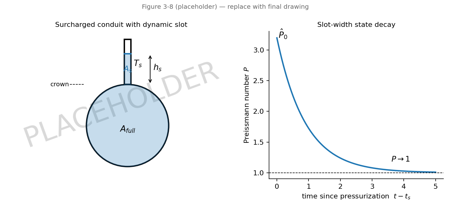
Figure 3-8 Conceptual representation of the dynamic Preissmann slot

The pressurization life cycle of a conduit end under the dynamic slot is summarized in Figure 3-9.

stateDiagram-v2
    direction LR
    FS : Free surface
    FS : slot closed, geometry from section tables
    PR : Pressurizing
    PR : depth crosses crown, state seeded P = P_hat_0
    SA : Slot active
    SA : width T_s from P, incremental A_s accumulation
    DP : Depressurizing
    DP : head falls below crown with hysteresis band
    FS --> PR : h rises past y_full
    PR --> SA : first pressurized iteration
    SA --> SA : P decays toward 1 over DPS_DECAY_TIME
    SA --> DP : h_s drops below hysteresis threshold
    DP --> FS : state reset, slot area released
    DP --> SA : head recovers before reset

Figure 3-9 State transitions of the dynamic Preissmann slot at a conduit end (rendered diagram; states and transitions as implemented in updateDPSState)

Implementation. The dynamic slot is implemented in the dynamic wave solver (DWSolver in src/engine/hydraulics/DynamicWave.cpp): the per-iteration geometry override in applyDPSGeometry, the post-iteration Preissmann-number update in updateDPSState, the nodal smoothing in spatialSmoothP, and the celerity-based time step limit in getLinkStep. The option values are held in SimulationOptions (src/engine/core/SimulationOptions.hpp) and parsed in src/engine/input/handlers/OptionsHandler.cpp.

Reference: Sharior, S., Hodges, B.R., and Vasconcelos, J.G. (2023). "Generalized, Dynamic, and Transient-Storage Form of the Preissmann Slot." Journal of Hydraulic Engineering, 149(11), 04023046.

3.3.10 Virtual Junctions

A change in a pipe's grade with no change in its cross-section must be represented in the node-link scheme by splitting the conduit at a junction. That junction introduces two artifacts. First, its surface area is floored at the minimum value A_Smin of Equation 3-22, so the split reach carries artificial storage that smears transients — a recognized limitation of the practice of artificially discretizing conduits with intermediate junctions (Pachaly et al., 2020). Second, each conduit solves its own momentum equation against the shared node head, so the momentum flux arriving from the upstream conduit is not transmitted; the node acts as a small stagnation volume. A virtual junction removes both artifacts for the specific case the practice is meant to serve: two collinear conduits of identical cross-section meeting at a grade break.

Virtual junctions are declared in a dedicated [VIRTUAL_JUNCTIONS] input section whose entries carry a name, an invert elevation and an optional maximum depth:

[VIRTUAL_JUNCTIONS]
;;Name           Elev        MaxDepth
VJ1              101.25
VJ2              100.80      4.50

All hydraulic geometry is derived: the maximum depth used by the solver equals the shared pipe's full depth, and the surcharge depth and ponded area are zero. In reports and output files a virtual junction appears as an ordinary junction whose stored volume is identically zero.

The optional third entry, MaxDepth, is a drawing property only. A virtual junction's derived maximum depth is the pipe crown, so a profile or section view that draws the ground surface at invert + maximum depth would sink the terrain to the crown at every break point. Supplying MaxDepth gives such views the real ground elevation to draw instead. No part of the solver, the routing, the reporting or the binary output file reads it, so a model produces identical results whether or not it is supplied; when it is omitted, viewers fall back to the pipe crown. A virtual junction created by splitting a conduit inherits a MaxDepth interpolated between the two end nodes' ground elevations.

A node is eligible to be a virtual junction only if it satisfies all of the following, which are enforced when the input file is processed:

Exactly two links are attached, and both are conduits. Pumps, orifices, weirs and outlets require a regular junction.
The two conduits have identical cross-sections — the same shape, dimensions, shape curve reference and number of barrels. Their Manning roughness values may differ, since a grade break often coincides with a change of pipe material.
Both conduit offsets at the node are zero; the node's invert is continuous with both conduit inverts.
The node is not a two-dimensional surface coupling point. A virtual junction has no opening, so it cannot exchange water with an overlying surface mesh. Point lateral inflows — external and dry weather inflows, RDII, subcatchment outlets, LID drains and the runtime lateral-inflow API — are permitted; see Lateral inflows below.
The routing method is dynamic wave (or the finite-volume method of Chapter 8, under which a virtual junction is consumed at mesh construction and becomes an ordinary interior face).

Violating any rule produces an input error naming the offending node.

Continuity treatment. A virtual junction is a sealed, zero-storage node. Its head is updated with the free-surface formula 3-15 using the natural half-link surface area contributed by its two conduits, without the minimum surface-area floor of Equation 3-22 — the floor is precisely the artificial storage the feature removes, while the natural link area is the correct linearization of the adjacent conduits' own storage response. When that natural area vanishes — a dry pair, or a fully surcharged pair whose slot width is small — the update falls back to a pure flow-balance (zero-storage) form of the surcharge update, Equation 3-28 with α = 1 and no surface-area floor, including the β crown-proximity blending so that entry into and exit from surcharge remains smooth. At convergence the flow balance \(\sum Q = 0\) holds at the node with no storage term. The node is sealed: its head may rise above the pipe crown without bound (like a manhole with a bolted cover), it can never flood or pond, and its committed volume and overflow are identically zero, so it contributes nothing to the system's storage or flooding totals.

Momentum treatment. When the pair has a through orientation — one conduit entering the node and one leaving — the solver couples the two momentum equations across the break. When flow runs in the pair's forward direction, the downstream conduit's upstream-weighted area and hydraulic radius (Equations 3-19 and 3-20) take the upstream conduit's mid-reach values as their upwind state, carrying the advected momentum state across the node instead of restarting it. This upwinding of the advected state is the whole of the momentum treatment: a virtual junction transmits no cross-junction convective momentum flux.

Retired option. The VIRTUAL_JUNCTION_MOMENTUM FULL setting formerly added the cross-junction convective correction of Equation 3-43 to the \(\Delta Q_{inertia}\) term of both conduits:


\[\Delta Q_{j} = \mathrm{\Delta}t\,\sigma_{j}\frac{\left( \overline{U}^{2}\overline{A} \right)_{dn} - \left( \overline{U}^{2}\overline{A} \right)_{up}}{\Lambda}, \qquad \Lambda = \frac{L_{up} + L_{dn}}{2}\]		(3-43)

It is retired as of 2026-08-14. For steady discharge \(\Delta\left( U^{2}A \right) = - U^{2}\Delta A\), so this correction carries the opposite sign to the per-conduit convective term it was meant to supplement, and adding it to both adjacent conduits applied it roughly three times over. On the SWASHES macdonald-periodic benchmark it destroyed 224–325 % of the routed volume; negating it restored mass conservation but still left a profile error of 5.24 % against 0.163 % for BASIC and 0.141 % for ordinary junctions. The keyword is still accepted, issues a warning, and is treated as BASIC. Models that need genuine momentum transport through a subdivided reach should use the finite-volume solver, which on the same benchmark is roughly 60× more accurate and 2.6× faster.

Pairs in a sag or peak orientation (both conduits pointing into, or out of, the node) receive the zero-storage continuity treatment but not the directional momentum coupling. The two conduits of a pair are also always solved together: neither is frozen by the converged-node bypass of the solution procedure unless both are, and the variable time step includes a pair-level Courant check \(\Lambda/\left( \left\lvert \overline{U} \right\rvert + c \right)\) in addition to the per-conduit checks of Section 3.4.

As a measure of how well the interface conserves momentum, the solver accumulates a discrete momentum residual for each through pair at the end of every routing step,


\[R_{j} = \left( \frac{Q^{2}}{A} \right)_{up} - \left( \frac{Q^{2}}{A} \right)_{dn} + g\overline{A}\left( Y_{up} - Y_{dn} \right)\]		(3-44)

evaluated per barrel at the two conduit ends meeting the node, and reports its maximum and mean in a Virtual Junction Summary in the status report. With identical cross-sections and a shared node head the hydrostatic terms cancel, so R_j measures the discrete momentum-flux mismatch directly.

Lateral inflows. A point lateral inflow at a virtual junction is integrated exactly as at any other node: it enters the flow balance \(\sum Q\) of the zero-storage update, so at convergence the downstream conduit carries the upstream discharge plus the lateral. The node stays sealed — a lateral that exceeds the pair's capacity raises the head above the crown without flooding or ponding, as a tap into a buried main would — and its committed volume remains zero. One guard is added. At a dry pair the natural half-link area vanishes and \(\sum \partial Q/\partial H\) is zero, so an imposed inflow would either divide a finite volume by nothing or fall into the dry-pair hold and be swallowed. While the node carries a lateral its surface area is therefore floored at a wetting floor: the pair's own natural half-link area evaluated at a seed depth of 2 % of the pipe's full depth, \(w(0.02\,y_{full})\,(L_{up}+L_{dn})/2\) per barrel. The floor is continuous with the natural area (the larger of the two is used) and inert once the pair is wetter than the seed depth, so it scales with the reach instead of introducing the fixed A_Smin storage the feature removes. Unfed virtual junctions keep their unfloored arithmetic. The momentum coupling is unchanged: the upwinding of Equations 3-19 and 3-20 hands the upstream conduit's state across the node, so with a lateral the treatment is first order in \(q_{lat}/Q\) — the same class of approximation a regular junction makes for all of its momentum — and the residual R_j of Equation 3-44 is legitimately nonzero at a fed node, which the Virtual Junction Summary marks. Under the finite-volume method the lateral is divided equally between the two cells adjoining the spliced face as a zero-momentum source (Chapter 8, §8.6.2). Re-fusing a fed virtual junction removes its inflow rows and unassigns any subcatchment or LID drain that targeted it, exactly as deleting the node would.

Modeling implications. A virtual junction transmits streamwise momentum and is intended for grade breaks between near-collinear pipes, where the deflection angle is small and axial momentum conservation is exact to within discretization error. A plan-view bend imposes a wall reaction force that a one-dimensional interface cannot represent; bends should remain regular junctions with entrance and exit loss coefficients. Because a virtual junction stores no water, a long conduit may be subdivided with virtual junctions to increase spatial resolution without accumulating the artificial nodal storage that the same subdivision with regular junctions would introduce. Control rules may reference a virtual junction's depth, which is well defined; its volume is identically zero.

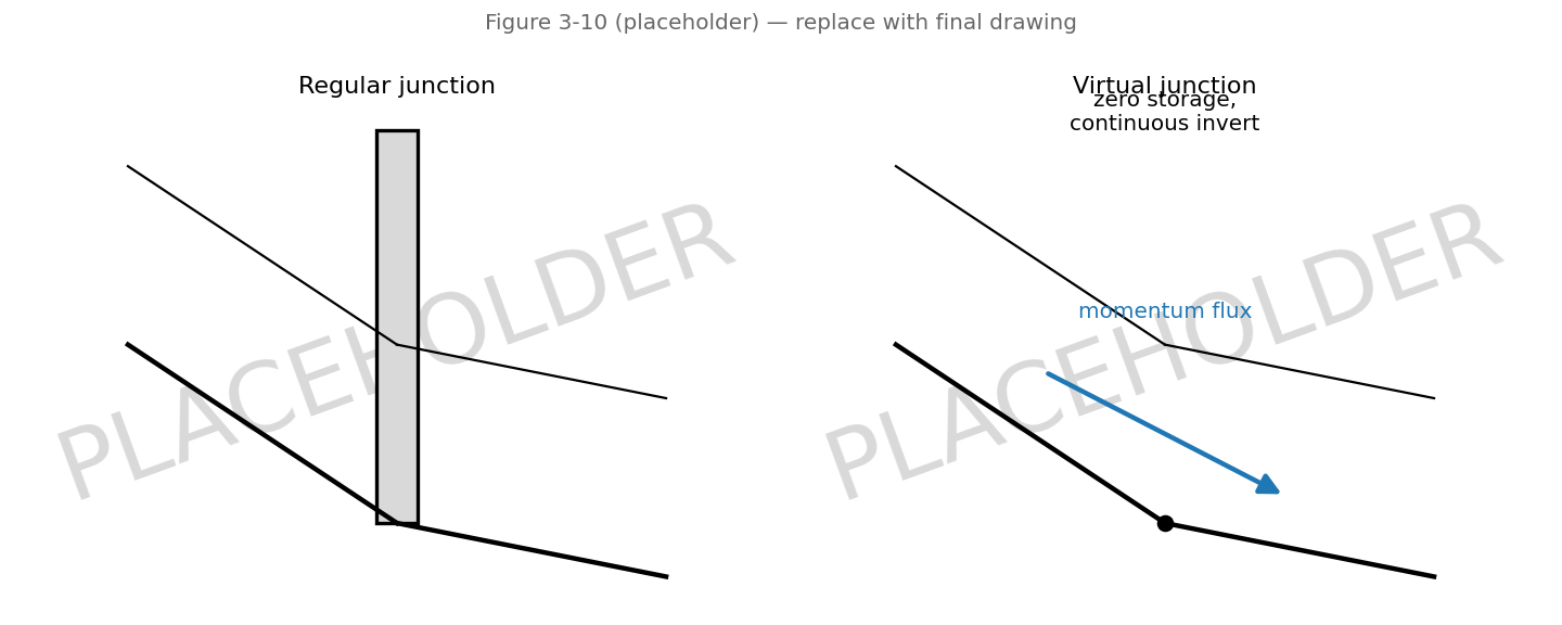
Figure 3-10 Virtual junction representation of a conduit grade break

Implementation. The solver-side pair table, per-iteration coupling cache, sealed node-depth update and momentum-residual diagnostic live in DWSolver (src/engine/hydraulics/DynamicWave.cpp: buildVirtualJunctionPairs, vjPrepareIteration, setNodeDepth, vjAccumulateResiduals). Eligibility validation and the split/fuse editing operations are shared between the input processor and the editing API in src/engine/edit/VirtualJunctionOps.cpp (vj_rule_violation), invoked from src/engine/input/PostParseResolver.cpp; the [VIRTUAL_JUNCTIONS] section is parsed in src/engine/input/handlers/NodesHandler.cpp.

Reference: Pachaly, R.L., Vasconcelos, J.G., Allasia, D.G., Tassi, R., and Bocchi, J.P.P. (2020). "Comparing SWMM 5.1 Calculation Alternatives to Represent Unsteady Stormwater Sewer Flows." Journal of Hydraulic Engineering, 146(7), 04020046.

Inlet junctions

An inlet junction is a virtual junction that also owns a street inlet. It is declared in its own [INLET_JUNCTIONS] section, whose first three entries mirror [VIRTUAL_JUNCTIONS] and whose remaining entries are the placement columns of [INLET_USAGE]:

[INLET_JUNCTIONS]
;;Name   Elev    MaxDepth  Inlet   CaptureNode  #Inlets  %Clog  Qmax  aLocal  wLocal  Placement
IJ1      98.00   0.50      Curb1   MH2          1        10     0     0       0       ON_GRADE

The node obeys every virtual-junction eligibility rule above and, in addition, both attached conduits must carry a STREET cross-section (error 623), the inlet design must exist (625), the capture node must exist, differ from the junction and be a real node (627), neither attached conduit may itself carry an [INLET_USAGE] row (629), the row may carry no extra entries (631), and an inlet junction without a usage row is refused (633). A design incompatible with the host section is a warning (635) that disarms the inlet, as in legacy SWMM.

Capture. At every routing step, after all other lateral inflows have been assembled and before the conduits are solved, the HEC-22 capture kernel computes the flow the inlet intercepts from the gutter flow arriving on the approach conduit — the conduit whose flow is directed toward the node; at a sag both conduits contribute — using the street geometry and the design dimensions exactly as for a conduit-attribute inlet. The captured flow leaves the junction as a negative lateral inflow and enters the capture node as a positive one; the bypass continues down the street. When the capture node floods, its overflow returns to the street through the inlet as backflow, so the transfer runs in either direction. Placement AUTOMATIC resolves by slope: the node is a sag when both conduits fall toward it, on-grade otherwise.

Continuity. Unlike a plain virtual junction the node is not sealed: water that rises above the street section leaves the corridor. The head update is the zero-storage virtual-junction form, but the flooding logic of an ordinary junction applies above a threshold equal to the street section's full depth or, when it is larger, the MaxDepth entry. MaxDepth can therefore raise the threshold — a raised curb line, a wall — but never lower it below the section, so a rendering-only rim inherited from a conduit split cannot make the node flood early. The node has no ponded area, so water above the threshold is lost as flooding. Its stored volume is identically zero: the half-link surface area it carries is the linearization of the adjacent conduits, not storage of its own.

Momentum. The pair receives the zero-storage continuity treatment only. The directional momentum coupling (the upwind-state carry-over across the break) is disabled at an inlet junction, because that coupling assumes a sealed pair with no lateral exchange at the node.

Routing methods. Inlet junctions require dynamic wave routing. Under kinematic or steady routing the virtual-junction rule applies (error 619); under finite-volume routing, which splices virtual junctions out of its mesh (§8.6.2), an inlet junction is also refused with error 619, because the spliced node could no longer carry the capture sink.

Results and files. The node reports as a JUNCTION in the output file. The Street Inlet Flow Summary lists it as NAME (node) beside the conduit-attribute inlets, with the same performance columns. When a model is written for a SWMM 5.x engine (the SWMM5 write profile of swmm_model_write_compat), an inlet junction is downgraded to an ordinary junction plus an [INLET_USAGE] row on its approach conduit with the same design and capture node — the legacy-equivalent model — and the writer reports the substitution.

Implementation: src/engine/hydraulics/Inlet.cpp (the kernel and the per-step transfer, inlet::InletSolver::computeAll), the unsealed flooding branch of DWSolver::commitNodeDepthState and the mechanism-1-only guard in DWSolver::vjPrepareIteration (src/engine/hydraulics/DynamicWave.cpp), validation in src/engine/input/PostParseResolver.cpp (validate_inlet_junctions), and the split/fuse editing operations ij_split_conduit / ij_fuse in src/engine/edit/VirtualJunctionOps.cpp.

3.3.11 Two-Component Pressure Approach (`SURCHARGE_METHOD TPA`)

All three surcharge treatments described so far share one fidelity limit: a head below the pipe crown is always reinterpreted as a free surface, so a sealed conduit cannot hold sub-atmospheric pressure during a rapid downsurge. OpenSWMM provides a fourth surcharge treatment, SURCHARGE_METHOD TPA, a pragmatic port of the two-component pressure approach of Vasconcelos, Wright and Roe (2006) to the node-link scheme. (Its natural home is the finite-volume solver, where the full shock-capturing formulation is available as FV_PRESSURE_CLOSURE TPA — Chapter 8.) Like DYNAMIC_SLOT it is flagged experimental.

Requirements. The method needs a closed conduit with a defined full depth: an open cross-section, or one whose \(Y_{full}\) is zero, never latches and keeps ordinary free-surface geometry — the option is inert outside closed pipe, so mixed networks need no special arrangement. Setup is the pair SURCHARGE_METHOD TPA and TPA_CELERITY under FLOW_ROUTING DYNWAVE. Only a sealed conduit end — a virtual junction (Section 3.3.10) or a node with positive surcharge depth — can hold sub-crown pressure; every other end vents. Signed heads reach the binary output only under REPORT_SIGNED_HEADS YES, and NODE_CONTINUITY SEMI_IMPLICIT (Section 3.5) is the recommended pairing.

Above the crown: a constant-width slot. Where the static slot of Section 3.3.6 uses the Sjőberg width function 3-30, TPA uses the classical celerity-derived width directly, held constant per conduit:


\[w_{tpa} = \frac{gA_{full}}{a^{2}}\]		(3-49)

where \(a\) is the acoustic celerity given by the TPA_CELERITY option, in project length units per second (converted internally; compare Equation 3-29). There is no Sjőberg decay and no clamp above 1.78 Y_full; the crown cutoff at Y/*Y*_full = 0.985257 applies as it does for the other slot methods. Above the crown this is the whole story: heads are always updated through the ordinary free-surface continuity formula with the slot supplying the surface area, and the surcharge branch of Equation 3-28 is never invoked.

Below the crown: the sub-atmospheric latch. The new capability is a per-conduit pressurized latch, recording whether the air pathway to the conduit has been cut — physical history, not a numerical device. The latch is set when the conduit reaches full (both end depths at Y_full, the same condition that engages the slot branch today). While it is set, a head below the crown at a sealed end does not revert the conduit to free-surface geometry: the flow area follows the signed slot line \(A_{full} + w_{tpa}(Y - Y_{full})\) — "shrinkage" of the section under negative gauge pressure — the top width stays \(w_{tpa}\), the hydraulic radius stays at its full-conduit value (the slot carries no wetted perimeter), and each end contributes \(w_{tpa}L/4\) of surface area to node continuity. Momentum needs no new terms: the solver already differences node heads, and a sub-crown head at a sealed node is simply a head — the latch's only job is preventing the geometry tables from reinterpreting it as a free-surface depth.

The latch is cleared when air can actually re-enter: at a vented end whose flow depth stands below the crown at that end (an unsubmerged opening — a vented node whose water level stands above the crown holds the column, exactly as a submerged inlet holds a siphon), or on column separation, when the mid-reach depth falls more than 30 ft below the crown — about one atmosphere of water column, past which a vapor cavity forms and two-phase dynamics outside the model's scope take over. Sealed means a virtual junction (Section 3.3.10) or a node with a positive surcharge depth (a bolted cover); everything else is vented. The latch is updated once per routing step, before the iterative solution begins, so the Picard iteration of Section 3.2 iterates a fixed operator — the same reasoning that has the dynamic slot advance its state between iterations rather than within them. When Anderson acceleration (Section 3.6) is active, the end nodes of any conduit whose latch changed this step take the plain iterate for that step, since a latch transition is a discrete operator switch (see Table 3-2).

What is and is not captured. DW node depths are floored at zero, so the vacuum representable at a node is bounded by the distance from the crown down to the node invert: stations that would fall below their own invert under vacuum — the deep sub-atmospheric transients of the negative-pressure siphon class — are finite-volume territory (Chapter 8). DW TPA's value is sealed sub-crown behavior: no spurious geometry flip, no spurious flooding, and a head that recovers smoothly when inflow returns. On the rapid-filling laboratory case of Vasconcelos et al. (2006), DW TPA's bore arrival lands within 2 % of the finite-volume timing (10.25 s against 10.45 s), where the Sjőberg static slot arrives about 20 % early (8.35 s) — measured on the mixed-flow closure study of issue #156. Phase 6 of that study, scoring against the digitized laboratory record on a shared absolute threshold (head first exceeding 0.15 m at the 9.9 m station, measured at 6.69 s), places the columns in absolute terms: the dynamic slot lands 0.14 s early (6.55 s), the static slot at 9.95 s, DW TPA at 12.25 s, and EXTRAN at 14.35 s — so DW TPA's agreement with the finite-volume timing above is scheme consistency, not accuracy on this filling case (and the finite-volume columns' own timing there is compromised by a documented initial-condition seeding defect). On the negative-pressure siphon case, Phase 6 measured every dynamic-wave column bottoming at 0.231–0.233 m of crest head against 0.1035 m for finite-volume TPA — the quantified form of the invert-floor limit above. To observe signed heads in the binary output file at all, set REPORT_SIGNED_HEADS YES (default NO preserves legacy bit-parity; the HEAD field then carries the true signed head while DEPTH stays floored — both solvers honor the option).

The method adds one [OPTIONS] keyword beside SURCHARGE_METHOD:

Key	Default	Meaning
`TPA_CELERITY`	100	Acoustic celerity \(a\) in Equation 3-49, in project length units per second. Air content can cut the true value by an order of magnitude, so it is a user parameter, exactly like the finite-volume solver's `FV_SLOT_CELERITY`.

NODE_CONTINUITY SEMI_IMPLICIT (Section 3.5) is the recommended pairing: with the constant \(w_{tpa}\) surface area the unified update is smooth through the crown.

Implementation. The latch update and geometry override are updateTpaLatch and applyTpaGeometry in DWSolver (src/engine/hydraulics/DynamicWave.cpp), hooked beside the dynamic slot's applyDPSGeometry; the per-conduit width (3-49) is computed at initialization. Gates: tests/unit/engine/test_dw_tpa.cpp.

Reference: Vasconcelos, J.G., Wright, S.J., and Roe, P.L. (2006). "Improved Simulation of Flow Regime Transition in Sewers: Two-Component Pressure Approach." Journal of Hydraulic Engineering, 132(6), 553–562.

3.3.12 Unsteady Friction (`UNSTEADY_FRICTION`)

Mixed-flow models that carry only steady friction reproduce observed transient damping only by inflating Manning's n to unphysical values. OpenSWMM offers the remedy of Pinto, Vasconcelos and Soares (2025) — a modified Vítkovský et al. (2000) instantaneous-acceleration term with a Brunone-type coefficient k₃ — as an option orthogonal to the surcharge method and shared with the finite-volume solver (Chapter 8). The friction slope becomes \(S_f = S_{fs} + S_{fu}\) with the steady term unchanged and


\[S_{fu} = \frac{k_{3}}{g}\left( \frac{\partial V}{\partial t} + c\,\mathrm{sgn}(V)\left\lvert \frac{\partial V}{\partial x} \right\rvert \right)\]		(3-50)

where the celerity c is regime-dependent: the acoustic celerity when the conduit is pressurized, the gravity-wave celerity otherwise. In this solver both come out of the mid-reach top width already in hand — the slot width while surcharged under a slot method (so TPA_CELERITY governs under TPA), the free-surface width otherwise, and the near-crown width under EXTRAN, which has no acoustic celerity of its own and is therefore the weakest pairing.

The term drops into the flow updating formula 3-14 the way every other term does. The local-acceleration half integrates semi-implicitly — k₃ joins the denominator alongside \(\Delta Q_{friction}\) and \(k_{3}\overline{A}\,V^{old}\) joins the numerator — which also enters the flow gradient 3-27, keeping the surcharge iteration and the semi-implicit node continuity consistent with the flow update. The convective half is an explicit term built from the end velocities. Two details are consequences of the node-link discretization rather than choices:

The velocity gradient uses a cross-link stencil. Within a single link the gradient estimator is the end-velocity difference, which is structurally zero on a full conduit (equal end areas) — exactly the pressurized case the term exists for. The gradient therefore reads the neighboring conduits' previous-iterate velocities across simple two-conduit junctions, sign-mapped into the link's frame, with the within-link difference as the fallback. The modeling consequence: unsteady-friction damping requires a discretized reach. A single long conduit has no neighbors to difference against and receives added inertia only; subdividing the reach (virtual junctions serve well, Section 3.3.10) restores the damping term.
Force mains have equal end areas by construction, so the gradient term vanishes and only the local-acceleration fold acts.

As in the finite-volume implementation, a 0.01 ft/s velocity dead-band keeps the added inertia from amplifying numerical settling noise, a per-step clamp bounds the update to half the incoming momentum, and with UNSTEADY_FRICTION NONE (the default) the original expressions are evaluated verbatim for bit-parity.

Fidelity expectations must be set honestly: the node-link solver cannot reproduce waterhammer (a 1255 m/s valve-closure transient is finite-volume-with-implicit-acoustics territory). The dynamic wave value proposition is better damping of inertial oscillations and post-surcharge transients at ordinary routing steps.

Key	Default	Meaning
`UNSTEADY_FRICTION`	`NONE`	`NONE` or `VITKOVSKY`. `NONE` is bit-inert in both solvers.
`UF_K3`	0.015	Brunone-type coefficient k₃ in Equation 3-50, used only when the method is not `NONE`. Paper-calibrated range 0.005–0.020, swept to 0.045.

Implementation. The dq-term extension lives in processManningLink and processForceMainLink of DWSolver (src/engine/hydraulics/DynamicWave.cpp), with the cross-link stencil tables built in DWSolver::init. Gates: tests/unit/engine/test_dw_unsteady_friction.cpp.

Reference: Pinto, S.I.G., Vasconcelos, J.G., and Soares, A.K. (2025). "Unsteady Friction in Mixed-Flow Models Based on the Saint-Venant Equations." Journal of Hydraulic Engineering, 152(1), 04025046.

3.4 Numerical Stability

The numerical stability of SWMM's dynamic wave results can be affected by the choice of the simulation time step. Numerical instability is characterized by oscillations in flow and water surface elevation that do not dampen out over time. Another indicator of numerical instability is a node which continues to "dry up" on each time-step despite a constant or increasing inflow from upstream sources.

Aside from examining the results for each conduit and node, SWMM 5 provides two metrics in its Status Report that can help determine if a solution shows signs of instability. One is the overall flow continuity error for the system. This is the difference between inflow and outflow for the entire system over the duration of the simulation. If this number is greater than 5 to 10 percent then the cause may be numerical instability (although other factors can affect the continuity error as well).

A second metric is a link's Flow Instability Index (FII). This index counts the number of times that the flow value in a link is higher (or lower) than the flow in both the previous and subsequent time periods. The index is normalized with respect to the expected number of such 'turns' that would occur for a purely random series of values and can range from 0 to 150. The Status Report identifies the links having the five highest FII's. Unfortunately since the FII does not take into account the magnitude of the flow fluctuations it cannot determine whether the instability is of engineering significance or not.

Stable explicit solutions of the St. Venant equations require that the time step be no longer than the time it takes for a dynamic wave to travel the length of the conduit (Cunge et al., 1980). This is known as the Courant-Friedrichs-Lewy (CFL) condition and can be expressed as:

\[\mathrm{\Delta}t \leq \frac{L}{\left| \overline{U} + c \right|}\]

(3-30)

where c is the wave celerity given by:

\[c = \sqrt{g\frac{\overline{A}}{\overline{W}}}\]

(3-31)

An equivalent form of this condition can be written as:

\[\mathrm{\Delta}t \leq \frac{L}{\left| \overline{U} \right|}\left( \frac{Fr}{1 + Fr} \right)Cr\]

(3-32)

where Fr is the flow's Froude number (see Equation 3-17) and Cr is the Courant number. The latter serves as an adjustment parameter that determines how conservative (Cr < 1) or liberal (Cr > 1) one wishes to be in strictly meeting the CFL condition (Cr = 1).

Although the SWMM 5 solution method uses an iterative implicit procedure in time to update flows and heads, it does so one conduit and node at a time, not simultaneously. There is no spatial coupling between elements as would occur in an unconditionally stable implicit solution scheme. Thus the CFL condition would still apply but perhaps not as strictly (by allowing one to use a Cr value greater than 1).

One can estimate a ∆t for each conduit by using the conduit's full depth Y_full in place of \(\frac{\overline{A}}{\overline{W}}\) in Equation 3-31 and ignoring the velocity in Equation 3-30. The solution time step would then be determined by the conduit with the smallest value of \(\frac{L}{\sqrt{gY_{full}}}\) . Short conduits lead to small time steps and longer computational times. Time steps of 10 to 30 seconds should suffice for conduit lengths of 200 to 400 feet (the typical spacing between sewer manholes) and full depths from 1 to 4 feet.

An option is available to artificially lengthen short conduits so that the CFL condition for a given user-supplied time step ∆t is met. The modified length \(L'\) is given by

\[ L' = \max\{ L, \Delta t ( \sqrt{gY_{full}} + \frac{Q_{full}}{A_{full}} ) \} \]

(3-33)

where Q_full is the Manning's normal flow value (Equation 3-23) evaluated at full depth Y_full and A_full is the flow area at full depth. This modified length is used in place of the original length in the equations presented in section 3.4. To make the artificially lengthened conduit have a flow resistance equivalent to the original length, its slope S₀ and roughness coefficient n are adjusted so that the Manning equation produces an equal head loss across both the original and lengthened conduit for any given flow. The modified slope \(S_{0}'\) for the lengthened conduit is:

\[S_{0}' = S_{0}\sqrt{\frac{L}{L'}}\]

(3-34)

while its modified roughness \(n'\) is:

\[n' = n\sqrt{\frac{L}{L'}}\]

(3-35)

The conduit lengthening option is applied to all conduits whenever the user supplies a non-zero value for the "lengthening" time step to be used in equation 3-33. This time step does not have to be the same as the computational time step used to solve the dynamic wave equations.

Another option available in SWMM 5 is to have the program use a variable computational time step that is adjusted throughout the simulation. The user supplies values of the smallest allowable time step (∆t_min), the largest allowable time step (∆t_max) and a desired Courant number (Cr) to be met. At any time t, the next time step is computed from the smaller of:

The smallest value of

\[\frac{L}{\left| \overline{U} \right|}\left( \frac{Fr}{1 + Fr} \right)Cr\]

for all conduits with non-negligible Fr.

The smallest value of

\[\frac{0.25\left( H_{crown} - E \right)}{{\mathrm{\Delta}H}^{t}}\]

for all non-outfall nodes that are not surcharged.

The second condition guards against an excessive change in node head over a single time step. Both conditions are evaluated using the flow and head solutions found at time t ( \({\mathrm{\Delta}H}^{t}\) is the change in head found from the prior time step). The resulting time step is not allowed to be less than ∆t_min nor greater than ∆t_max. The initial time step used at time 0 is ∆t_min.

To illustrate these concepts consider a 2 ft x 2 ft rectangular conduit that is 2,000 ft long with a 0.05% slope and has a Manning's roughness of 0.015 (see Figure 3-5). When divided into 10 equal length sections of 200 ft each the estimated stable time step is \(\frac{200}{\sqrt{32.2 \times 2} = 25}\) seconds. When analyzed as just a single 2,000 ft long section it increases to 250 seconds.

Example1a.png

Figure 3-5 Profile view of example rectangular conduit (not to scale)

Figure 3-6 shows the outflow hydrographs for these two analysis options for a 1-hour sinusoidal inflow hydrograph with peak flow of 10 cfs (the dotted curve in the figure). Both results are completely stable. The option with the higher spatial resolution produces a more skewed hydrograph with a slightly lower peak.

image17

Figure 3-6 Outflow hydrographs for example conduit -I

Now consider what happens when the 10-section conduit is analyzed with a fixed time step of 120 seconds which is much larger than the stable fixed step of 25 seconds. As shown in Figure 3-7 the solution becomes completely unstable. When 120 seconds is used as the upper limit of a variable time step a stable result is produced. In this case SWMM's Status Report shows that the variable time step ranged from 24 to 120 seconds with the average being 42.

image18

Figure 3-7 Outflow hydrographs for example conduit – II

3.5 Semi-Implicit Node Continuity

The head updating scheme described in Sections 3.2 and 3.3.5 is a two-branch formulation: below the crown a node's head advances with the free-surface continuity formula 3-15, and above it the surcharge formula 3-28 takes over. The switch between the two occurs exactly at the crown elevation, so the head-update operator is discontinuous there. OpenSWMM offers an alternative single-branch formulation, selected with the NODE_CONTINUITY option:

Key	Values	Meaning
`NODE_CONTINUITY`	`EXPLICIT` (default)	The classic two-branch formulation of Sections 3.2 and 3.3.5.
	`SEMI_IMPLICIT`	The unified formulation of Equation 3-45.

The semi-implicit formulation recognizes that the flows entering the head update of Equation 3-15 themselves depend on the head being solved for. Linearizing the net nodal flow about the current head estimate using the flow gradients of Equation 3-27, \(\sum Q^{t + \mathrm{\Delta}t} \approx \sum Q + \sum\frac{\partial Q}{\partial H}\mathrm{\Delta}H\), and carrying the correction into the trapezoidal head update yields a single equation used at every non-outfall node regardless of its surcharge state:


\[H^{t + \mathrm{\Delta}t} = H^{t} + \frac{\frac{\mathrm{\Delta}t}{2}\left( \sum Q^{t} + \sum Q^{t + \mathrm{\Delta}t} \right)}{\max\left( A_{S} + \frac{\mathrm{\Delta}t}{2}\sum\frac{\partial Q}{\partial H},\ A_{Smin} \right)}\]		(3-45)

where \(A_{S}\) is the node assembly surface area of Equation 3-22 and the flow derivatives are those computed during the flow update, exactly as in Section 3.3.5. When the surface area dominates the denominator the update reduces to the ordinary free-surface formula 3-15; as a node approaches and passes through surcharge the flow-derivative term takes on the role that the surcharge formula 3-28 plays in the explicit scheme, with the minimum surface area A_Smin bounding the denominator from below. The under-relaxation of Step 5 of the solution procedure and the ponding rules of Section 3.3.7 apply unchanged.

The practical consequence is that the head-update operator has no branch at the crown: a node passes into and out of surcharge through one smooth expression. This matters most in combination with the convergence acceleration of Section 3.6, whose validity depends on the smoothness of the iteration operator, and it is the recommended node continuity setting for models containing virtual junctions (Section 3.3.10).

Implementation. The unified branch is implemented in setNodeDepth of DWSolver (src/engine/hydraulics/DynamicWave.cpp); the option is declared in SimulationOptions (src/engine/core/SimulationOptions.hpp) and parsed in src/engine/input/handlers/OptionsHandler.cpp.

3.6 Anderson Acceleration of the Iterative Solution

The successive-approximation procedure of Section 3.2 is a fixed-point (Picard) iteration: each pass applies the same head-update operator to the latest head estimates until no head changes by more than the convergence tolerance. Fixed-point iteration converges linearly, and the relaxation factor θ = 0.5 that damps each update stabilizes the iteration without improving its rate. In networks with many tightly coupled nodes the solver can consume its full trial allotment on nearly every routing step even under mild conditions. OpenSWMM offers an optional acceleration of this iteration, enabled with:

[OPTIONS]
ANDERSON_ACCEL   YES        ;; default is NO

Let \(G\) denote the complete head-update operator for a node — the continuity solve of Equation 3-15, 3-28 or 3-45 together with the under-relaxation of Step 5 — and let \(H_{k}\) be the node's head estimate entering iteration k. The iteration residual is


\[r_{k} = G\left( H_{k} \right) - H_{k}\]		(3-46)

and convergence is declared when its magnitude falls within the head tolerance. Rather than simply accepting \(G\left( H_{k} \right)\) as the next iterate, Anderson acceleration of depth two (equivalently, Aitken's secant update) blends the two most recent operator outputs so as to cancel the residual predicted by a linear model of the iteration. The mixing coefficient is


\[\alpha_{k} = \min\left( 1,\ \max\left( 0,\ \frac{r_{k}\left( r_{k} - r_{k - 1} \right)}{\left( r_{k} - r_{k - 1} \right)^{2}} \right) \right)\]		(3-47)

and the accepted iterate is the convex blend


\[H_{k + 1} = \left( 1 - \alpha_{k} \right)G\left( H_{k} \right) + \alpha_{k}\,G\left( H_{k - 1} \right)\]		(3-48)

Clamping α_k to the interval [0, 1] restricts the update to interpolation between two already-computed, already-bounded operator outputs: when successive residuals shrink with the same sign the blend degenerates to the plain iterate \(G\left( H_{k} \right)\), and no extrapolated head can be produced. The blend is applied per node, beginning with the second trial of each routing step (the first trial has no history to mix). When a mixed head is accepted it is committed through the same routine as an ordinary update, so the node's volume, overflow and rate of depth change — quantities that feed flooding totals, the mass balance and the variable time step — always describe the head actually accepted. In practice the acceleration reduces trial counts by roughly 25 to 50 percent per routing step on networks that otherwise iterate to the trial limit.

The acceleration is justified only where the operator \(G\) is smooth — where small head changes produce proportionally small changes in the update. Two per-iteration safeguards enforce this. A residual-magnitude gate applies the blend only when \(\left\lvert r_{k} \right\rvert \leq 20\varepsilon\), where ε is the head convergence tolerance, since far from convergence the linear-iteration model underlying Equation 3-47 does not hold. And a mixed head that would be negative (below the node invert) is discarded in favor of the plain iterate. In addition, nodes at which the operator is known to be non-smooth are excluded from mixing for the current trial and simply take the plain iterate; Table 3-2 lists the exclusions. Note that surcharged junctions are excluded only under the EXPLICIT node continuity formulation, whose update switches branches at the crown; under SEMI_IMPLICIT (Section 3.5) the unified update of Equation 3-45 is smooth through the surcharge transition and surcharged junctions remain eligible for acceleration — one reason the two options pair well.

Table 3-2 Conditions under which Anderson acceleration reverts to standard iteration

Condition	Applies when	Reason
Surcharged node	`SURCHARGE_METHOD EXTRAN` with `NODE_CONTINUITY EXPLICIT`	The head update switches from Equation 3-15 to Equation 3-28 at the crown.
Active dynamic slot	`SURCHARGE_METHOD DYNAMIC_SLOT`; node touches a conduit with A_s > 0	The slot geometry of Section 3.3.9 is rewritten each iteration, so the operator differs between iterates.
Near the static slot cutoff	`SURCHARGE_METHOD SLOT`; node touches a closed conduit with \(0.98 \leq \overline{Y}/Y_{full} \leq 1.02\)	The slot width of Equation 3-30 engages abruptly at the crown cutoff.
TPA latch transition	`SURCHARGE_METHOD TPA`; node touches a conduit whose pressurized latch changed this routing step	A latch transition is a discrete operator switch (Section 3.3.11). Steadily latched or steadily free conduits remain eligible.
Weir or orifice at its crown	Upstream hydraulic grade line at or above the structure crown; both end nodes	The flow equation switches discontinuously (weir to orifice; partial to full submergence).
Pump end nodes	Always; both end nodes of every pump	Pump on/off status is discrete.

Finally, a node is counted as converged only when both the plain residual \(\left\lvert G\left( H_{k} \right) - H_{k} \right\rvert\) and the accepted movement \(\left\lvert H_{k + 1} - H_{k} \right\rvert\) are within the head tolerance. Testing accepted movement alone would let a blend that happens to land near the previous iterate declare convergence while the underlying flow balance is still unsatisfied; with acceleration disabled the two tests coincide and the criterion reduces exactly to that of Section 3.2.

Figure 3-11 summarizes one accelerated iteration.

flowchart TD
    A[Start iteration k] --> B[Compute plain iterate G of H_k for every node]
    B --> C[Evaluate residual r_k = G of H_k minus H_k]
    C --> D{Residual above 20 eps gate and node eligible per Table 3-2}
    D -- no --> E[Accept plain iterate H_k+1 = G of H_k]
    D -- yes --> F[Clamped mixing coefficient theta_k]
    F --> G[Two-point blend of current and previous iterate]
    G --> H{Blended depth negative}
    H -- yes --> E
    H -- no --> I[Accept blended iterate and re-commit canonical state]
    E --> J{Plain residual and accepted movement both within tolerance}
    I --> J
    J -- no --> B
    J -- yes --> K[Node converged]

Figure 3-11 Workflow of one Anderson-accelerated iteration of the successive-approximation loop (rendered diagram)

Implementation. The mixing update, the residual gate and the two-condition convergence test are implemented in updateNodeDepthsTeam of DWSolver (src/engine/hydraulics/DynamicWave.cpp), with the exclusion flags of Table 3-2 computed once per iteration in computeAASkipFlags and the canonical state commit in commitNodeDepthState. The option is declared in SimulationOptions (src/engine/core/SimulationOptions.hpp).

Table of Contents

3.1 Governing Equations

3.2 Solution Method

3.3 Computational Details

3.3.1 Average Cross-Section Properties

3.3.2 Surface Area Calculations

3.3.3 Inertial Damping

3.3.4 Flow Limitations

3.3.5 Surcharge Conditions

3.3.6 Preissmann Slot

3.3.7 Flooding and Ponding

3.3.8 Summary of Special Conditions

3.3.9 Dynamic Preissmann Slot

3.3.10 Virtual Junctions

Inlet junctions

3.3.11 Two-Component Pressure Approach (SURCHARGE_METHOD TPA)

3.3.12 Unsteady Friction (UNSTEADY_FRICTION)

3.4 Numerical Stability

3.5 Semi-Implicit Node Continuity

3.6 Anderson Acceleration of the Iterative Solution

3.3.11 Two-Component Pressure Approach (`SURCHARGE_METHOD TPA`)

3.3.12 Unsteady Friction (`UNSTEADY_FRICTION`)