 |
OpenSWMM Engine
6.0.0-alpha.4
Data-oriented, plugin-extensible SWMM Engine (6.0.0-alpha.4)
|
|
OpenSWMM Engine
6.0.0-alpha.4
Data-oriented, plugin-extensible SWMM Engine (6.0.0-alpha.4)
|
______________________________________________________________________________
Chapter 3 notes that although more powerful solution techniques are available — among them shock-capturing finite volume schemes (Toro, 2001) — SWMM 5 continues to use EXTRAN's node-link approach. This chapter documents the alternative OpenSWMM provides: a Godunov-type explicit finite-volume solver, selected with FLOW_ROUTING FV.
The finite-volume solver supplements rather than replaces the existing methods. Dynamic wave analysis (Chapter 3) remains the default and remains the right choice for most work. The finite-volume solver exists for the cases where the node-link formulation is structurally, rather than incidentally, limited: exact volume conservation, transcritical flow in steep sewers, and the speed of a pressurization front.
Dynamic wave analysis carries one discharge per conduit and treats a junction as a storage volume. Three consequences follow, and the finite-volume method addresses each:
Conservation. The dynamic wave momentum equation is written in a non-conservative form. Water volume is tracked well but not exactly, and the routing continuity error is a diagnostic the modeller is expected to watch. A finite-volume method in conservation form conserves volume identically — the flux that leaves one control volume is the same number that enters the next — so any continuity error that is reported arises from the reporting itself rather than from the solution.
In-conduit resolution. With one discharge per conduit, a backwater profile or a bore inside a pipe cannot be represented at all. The finite-volume mesh subdivides each conduit, so the flow field within a reach is resolved.
Discontinuities. Pressurization fronts, hydraulic jumps and transcritical transitions are genuine discontinuities. Their propagation speed is set by the Rankine–Hugoniot conditions, which only a conservative scheme reproduces (Hou and LeFloch, 1994). The dynamic wave solver handles transcritical flow by suppressing it, through inertial damping and normal-flow limiting.
Several aspects of the analysis remain unchanged: the method is still one-dimensional, still uses the Preissmann slot for pressurized flow under its default closure — which cannot represent sub-atmospheric pipe pressure; the optional TPA closure of §8.4.5 can — and still treats a general junction as a stagnation volume (§8.6).
The conservation form of the St. Venant equations for a channel or pipe of arbitrary but prismatic cross-section is
\[\frac{\partial A}{\partial t} + \frac{\partial Q}{\partial x} = q_{L}\] | Continuity | (8-1) | |
\[\frac{\partial Q}{\partial t} + \frac{\partial}{\partial x}\left( \frac{Q^{2}}{A} + gI_{1} \right) = gI_{2} + gA\left( S_{0} - S_{f} \right)\] | Momentum | (8-2) |
where \(A\) is flow area, \(Q\) discharge, \(q_L\) lateral inflow per unit length, \(S_0\) bed slope, \(S_f\) friction slope, and \(I_1\) is the first moment of the wetted area about the free surface,
\[I_{1}(h) = \int_{0}^{h}{(h - \eta)\,T(\eta)\,d\eta} = \int_{0}^{h}{A(\eta)\,d\eta}\] | (8-3) |
with \(T\) the top width and \(h\) the depth. The second equality follows by differentiating under the integral, and it is the form OpenSWMM tabulates: \(I_1\) is simply the antiderivative of \(A\). The term \(I_2\) accounts for width variation along the conduit and vanishes for a prismatic reach, which every SWMM conduit is.
Comparing (8-2) with the dynamic wave momentum equation (3-2), the difference is that the pressure and convective terms appear inside the flux divergence rather than as separate gradient terms. This placement of terms is what gives the scheme its conservation property.
The mesh is internal numerical discretization. It creates no named objects, appears in no report, and is invisible to the model's topology. Each conduit is divided into
\[n = \max\left( n_{min},\ \left\lceil L/\Delta x_{target} \right\rceil \right)\] | (8-4) |
cells of equal length, where \(\Delta x_{target}\) is FV_CELL_LENGTH and \(n_{min}\) is FV_MIN_CELLS. FV_MIN_CELLS is a floor and applies whether or not a \(\Delta x\) target is set.
The default is FV_MIN_CELLS 4, FV_CELL_LENGTH 0 — four cells per conduit with no length target. One cell per conduit is available but is not a supported operating point. A cell-centred scheme places the cell's bed at its mid-point elevation, so a conduit meshed as a single cell presents an artificial bed step of half the conduit's fall at every manhole. On the EPA reference drainage model, mean absolute peak-flow deviation from the dynamic wave solver against cells per conduit:
| cells per conduit | 1 | 2 | 4 | 8 |
|---|---|---|---|---|
| mean absolute peak-flow deviation | 37.1 % | 25.7 % | 15.3 % | 7.6 % |
| worst link | −75.8 % | −58.1 % | −43.2 % | −22.6 % |
| wall-clock, relative to one cell | 1.0× | 1.4× | 2.2× | 5.4× |
Four cells is a practical compromise rather than a converged result: it more than halves the one-cell error for about twice the cost, while further refinement improves accuracy more slowly than it adds cost. Set FV_CELL_LENGTH, or raise FV_MIN_CELLS, whenever peak flows or in-conduit profiles matter.
The conduit length used is the Courant-lengthened mod_length (Chapter 3), so LENGTHENING_STEP acts as a \(\Delta x\) floor for short pipes exactly as it acts as a length floor for the dynamic wave solver, and the bed slope and roughness the finite-volume solver uses are the same adjusted values.
The mesh is fixed after initialization. There is no adaptive mesh refinement; the solver adapts in time (§8.5.5) rather than in space.
Mixed free-surface and pressurized flow is handled with no regime-switching logic. The Preissmann slot is folded into the cross-section relations \(A(h)\), \(T(h)\) and \(R(h)\), producing one continuous geometry valid from dry bed to full pressurization. Every cell evaluates the same flux function, and a "transition" is simply a cell's depth crossing the crown.
The slot width is derived from the pressurized wave celerity the user asks for, rather than the other way round:
\[T_{slot} = \frac{g\,A_{full}}{c_{slot}^{2}}\] | (8-5) |
where \(c_{slot}\) is FV_SLOT_CELERITY. Making the celerity the user-facing quantity keeps the accuracy/cost trade explicit: because the explicit time step is bounded by \(\Delta x/(|v| + c)\), a physical acoustic celerity of 1000 ft/s or more would collapse the step size. The default of 100 ft/s is the same order the dynamic wave solver's SURCHARGE_METHOD SLOT produces. The slot is additionally capped at 5 % of the section's maximum width so it can never become the dominant storage and understate a surge.
Two practical consequences of (8-5) and the cap, measurable through the diagnostics of §8.7.1: the slot's share of stored volume scales as \(1/c_{slot}^{2}\), and requests below the cap-implied celerity \(\sqrt{g A_{full}/(0.05\,W_{max})}\) are inert — every such value produces byte-identical geometry (WARNING 108 reports the override). The cap-implied celerity is shape-dependent, since \(A_{full}/W_{max}\) varies by a factor of 2–3 across the closed-section catalog: for a circular pipe it is reached at \(c \approx 22.5\sqrt{D}\) ft/s (≈ 39 ft/s at D = 3 ft, ≈ 67 ft/s at D = 9 ft). Because the slot also absorbs part of the friction grade while engaged, steady full-bore head loss converges on the Manning value from below as the celerity rises (§8.7.1) — a low celerity understates surcharge and head loss together.
The slot does not appear abruptly at the crown. It opens smoothly over \([y_{c},\,y_{full}]\), with \(y_c\) the crown cutoff of Chapter 3 (0.985257 \(y_{full}\)), through a ramp \(\varphi\) that is \(C^{1}\) at both ends:
\[T(h) = T_{x}(h) + T_{slot}\,\varphi(s), \qquad s = \frac{h - y_{c}}{y_{full} - y_{c}}\] | (8-6) | ||
\[\varphi(s) = s^{2}(3 - 2s) \quad\text{for } 0 < s < 1\] | (8-7) |
where \(T_x\) is the section's own top width. A discontinuous \(dA/dh\) at the crown would produce spurious reflections there and corrupt the Riemann solver's wave-speed estimates; the taper is what prevents both. The area is the exact integral of (8-6), so \(A\) and \(T\) remain a consistent pair through the transition.
Open sections carry no crown and no taper: above y_full the section simply continues with vertical walls of width \(w_{max}\), which is one code path with the closed case and keeps the celerity physical.
Depressurization is the same mechanism in reverse — the cell's state re-enters the free-surface part of \(A(h)\) — and the closure is memoryless, so a pipe driven repeatedly over and back across the crown returns to the same state each time. This is why the static slot is used here rather than the Dynamic Preissmann Slot: a relaxing slot makes bore speed depend on relaxation history, which would destroy the Rankine–Hugoniot front speed the method exists to get right.
That argument rules out relaxing closures — ones whose pressurized celerity evolves with pressurization history, like the dynamic slot — and it is worth being precise that it does not rule out the TPA closure of §8.4.5. TPA's pressurized celerity is the same constant \(a\) as the static slot's, so the Rankine–Hugoniot speed of a filling bore is unaffected by its history flag; only the \(\Delta A < 0\) branch — the sub-atmospheric regime, which the static slot handles unphysically in any case — consults the flag at all.
The solver carries \(A\) and derives the free surface as \(\eta = z_b + h\), so it needs \(h(A)\). This inverse is constructed from the forward closure itself rather than from SWMM's Y-tables.
The reason is worth recording. SWMM's geometry tables are independent tabulations: A_Circ gives area from depth and Y_Circ gives depth from area, and they round-trip only to table resolution — measured at 0.016 ft on a 3 ft circular pipe near the crown, about 0.5 % of the diameter. That is harmless for the dynamic wave solver, which never composes them. Here it is not: cells at equal free surface but different bed elevation would reconstruct different surfaces, and the still-water property of §8.5.2 would fail on every partly-full pipe.
For the same reason, the tabulated top width is not the finite difference of the tabulated area. T is therefore used only where the physical top width is the quantity wanted — wave celerity and node surface area — while the flux path uses \(A\) and \(I_1\), which are mutually consistent by construction.
The inversion itself proceeds in three stages, all prepared at initialization from the forward closure:
\[h(A) = y_{full} + \frac{A - A_{crown}}{T_{slot}}, \qquad A \geq A_{crown}\] | (8-19) |
This inversion is the solver's hottest kernel: profiling a \(\Delta x\) = 20 ft run placed it and the closure evaluations it drives at 87 % of total solver time. The Brent construction replaced an earlier regula-falsi-only path at a measured 3.2× overall speedup with bit-identical results.
Implementation. The forward closure is openswmm::fv::kernels::areaOfDepth, openswmm::fv::kernels::widthOfDepth and openswmm::fv::kernels::i1OfDepth; the inversion is openswmm::fv::kernels::depthOfArea with the fallback openswmm::fv::kernels::depthOfAreaBracketed, all in src/engine/hydraulics/fv/FvKernels.hpp. The tables are the i1_tbl and h_tbl members of openswmm::fv::FvGeometry (src/engine/hydraulics/fv/NetworkMeshData.hpp, kI1Samples = 129), built in src/engine/hydraulics/fv/NetworkMeshBuilder.cpp.
Experimental. The option and the solver described here are fully functional and gated, but the pass cannot yet compose with the local-time-stepping macro cycle (§8.5.6) — tiering stands down on any substep where the solve engages — and the slot program's next round (R2b) is expected to revise it. The GUI surfaces it as an explicitly experimental checkbox on the Routing & Hydraulics page.
FV_PRESSURIZED_IMPLICIT YES removes the slot's wave from the explicit time-step law. Above the taper band the closure (8-4) is exactly linear in head, so the acoustic pair — slot storage \(T_{slot}\,\partial H/\partial t\) against the pressure gradient \(gA\,\partial H/\partial x\) — is a linear diffusion system in \(H\) that can be integrated implicitly ( \(\theta = 1\)), unconditionally stably. Each substep, every closed- section cell at or above the band entry \(y_c\) forms, with its like neighbours, a symmetric positive-definite head system
\[\frac{T_i\,\Delta x_i}{\Delta t}H_i + \sum_f C_f\,(H_i - H_{nbr}) = \mathrm{RHS}_i,\qquad C_f = \frac{\alpha_f\,\Delta t\,g\,\hat A_f}{L_f},\quad \alpha_f = \frac{1}{1+\Delta t\,\gamma_f}\] | (8-24a) |
solved directly — the Thomas algorithm along pipe chains, Jacobi- preconditioned conjugate gradients where a folded junction has three or more branches. The solve is a flux predictor: the back-substituted face discharges overwrite the face mass fluxes, and the ordinary cell and node updates then integrate them unchanged, so mass conservation, step rejection, hot start and reporting are structurally untouched. Membership is a pure function of the instantaneous state — no flags, no memory — so the hysteresis and hot-start properties of §8.4 are inherited rather than re-proven. (Under the TPA closure of §8.4.5 membership is instead the regime flag, which is fixed within a substep; see that section for the interaction.)
Three details carry the accuracy claims. First, the conductance area \(\hat A_f\) and the friction coefficient \(\gamma_f\) use the conveyance area \(\min(A, A(y_{full}))\) — the slot stores volume but must not conduct, the same distinction the dynamic wave solver draws when it strips the slot from conveyArea. At steady state (8-24a) then reduces per face to \(\Delta H/L = -S_f\) exactly, which makes full-bore head loss equal to the friction law and independent of FV_SLOT_CELERITY — where the explicit scheme understates it at low celerity (§8.4.1). Second, pressurized algebraic junctions whose every face joins two pressurized states are folded into the system as unknown rows (a lagged junction head would recreate the very feedback stiffness the solve removes); a solved head that violates the node's rim or invert is demoted to a Dirichlet row at the clamp and the imbalance books through the carry ledger into the same flooding and ponding paths as always. Third, transition faces — one side pressurized, one free — stay entirely explicit, Godunov flux and Courant bound alike: filling bores keep their shock-captured physics at a front-resolving step, and the step census drops the celerity of a pressurized side only where the face is covered by the solve. A fully pressurized network therefore runs at the advective bound — the slot width becomes a pure accuracy parameter with no runtime price — while a network that never pressurizes is bit-identical with the option on.
The pass lives in src/engine/hydraulics/fv/PressurizedHeadSolver.{hpp,cpp} and runs on the CPU solver's global path (a device backend request is overridden while the option is on; composing the solve with the local- time-stepping macro cycle is future work). Gates: tests/unit/engine/test_fv_pressurized_implicit.cpp.
FV_PRESSURE_CLOSURE TPA)Experimental. Fully functional and gated, selected with
FV_PRESSURE_CLOSURE TPA; the defaultSLOTpreserves the closure of §8.4.1–§8.4.2 bit for bit. One known limitation is pinned in-tree (high-celerity filling, below).
The slot closure is monotone: a head below the crown is a free surface, so a full pipe carrying pressure below atmospheric has no representation — a sealed reach hit by a rapid downsurge spuriously reverts to free-surface geometry instead of holding vacuum. The two-component pressure approach of Vasconcelos, Wright and Roe (2006) lifts exactly this restriction: pressure is decomposed into a hydrostatic component, present in both regimes, and a surcharge component \(h_s\) carried only by a pressurized cell, and \(h_s\) may be negative — the pipe stays full, at sub-atmospheric pressure, until air can physically reach it.
Requirements. TPA applies to closed conduits only: a cell whose cross-section is open never latches (updateTpaFlags clears its flag unconditionally) and evaluates the free-surface closure verbatim, so mixed networks need no special arrangement — the option is inert outside closed pipe. Eligibility needs nothing beyond the closed section's own full-flow properties, which every closed shape already carries for the SLOT closure: \(A_{crown}\), \(y_{full}\), and the slot width \(T_{slot} = gA_{full}/a^{2}\). Setup is FLOW_ROUTING FV with FV_PRESSURE_CLOSURE TPA; the acoustic celerity \(a\) comes from FV_SLOT_CELERITY (§8.4.1). A node is sealed against the venting sweep by a positive SURCHARGE_DEPTH (a bolted cover); virtual junctions are sealed by construction (§8.6.2). Sub-atmospheric heads reach the .out file only under REPORT_SIGNED_HEADS YES — without it the physics is computed but invisible, the HEAD field flooring at the invert. The validated configuration for the sub-atmospheric class is the explicit scheme with forward-Euler time integration or the implicit acoustic solve (see the scoring below); FV_TIME_INTEGRATION RK2 alters the stability landscape in both directions and is not a safe default with TPA (see the known limitation).
The closure pair. The observation that makes TPA cheap here is that the existing slot line is the TPA pressurized branch for \(\Delta A = A - A_{crown} \geq 0\). TPA extends the same line to both signs of \(\Delta A\):
\[h(A) = y_{full} + \frac{A - A_{crown}}{T_{slot}}, \qquad h_{s} = h - y_{full} \text{ of either sign}\] | (8-34) | ||
\[I_{1}(h) = I_{1,crown} + A_{crown}\,\left( h - y_{full} \right)\] | (8-35) |
Equation (8-35) is the paper's Eq. (12b): the pressurized first moment drops the \(\tfrac{1}{2}T_{slot}(h - y_{full})^{2}\) term the SLOT closure keeps — that term is the slot's own numerical storage pressure, not part of the physical decomposition. Free-surface cells evaluate the table closure of §8.4.2 unchanged, including the tapered slot mouth; the two branches are continuous at \(A = A_{crown}\). The pressurized celerity is the constant \(a\), the hydraulic radius stays frozen at \(r_{full}\), and the pressurized inverse \(h(A)\) is closed-form. FV_SLOT_CELERITY doubles as the TPA acoustic celerity \(a\) — it is the same physical dial, since \(T_{slot} = gA_{full}/a^{2}\) is derived from it under either closure.
The regime flag is physical air-pathway history, not numerical relaxation. Which branch a cell evaluates is decided by a per-cell flag recording whether air can reach the cell — the paper's governing rule. Its transitions, applied once per substep outside the flux loops:
Venting. A cell has atmosphere contact when one of its faces touches an unsealed node — no SURCHARGE_DEPTH seal — whose water level at that face stands below the pipe crown, or a free-surface neighbouring cell whose surface stands below the shared crown. The submergence check is load-bearing: air cannot enter through an opening that is itself under water, and without the check every sealed reach unzips from its vented ends (measured — the sealed-siphon fixture drained and then diverged). Two alternative rules were measured and rejected rather than assumed away: the paper's literal unconditional venting of the regime-transition interface unzips a submerged pressurized leg through a chain of momentary exits, and an entry-at- \(A_{full}\) island rule broke the V-shaped filling case. Virtual junctions need no special casing and get the correct physics by construction: a virtual junction is spliced out of the mesh (§8.6.2), so it can never seed the venting sweep — a splice has no atmosphere contact — while contact still propagates across it, because cell chains span the splice.
Interaction with FV_PRESSURIZED_IMPLICIT (§8.4.4). The pressurized branch (8-34) is the same linear closure the implicit solve exploits, so the two options compose, with four TPA-specific rules. Membership in the implicit set is the regime flag — a latched cell with \(h_s < 0\) sits below the crown yet is exactly the stiff-acoustic case the solve exists for — and since the flag is fixed within a substep, the SPD structure is unchanged. A sealed node standing against a flagged interior cell presents a pressurized ghost even though its head is below the crown. The Dirichlet floor applied to a folded junction row extends below the node invert by the column-separation bound, because a solved sub-atmospheric head is now legal. And a flagged cell's storage row uses the regime's own width \(T_{slot}\) at any head, never the free-surface table width — the measured failure without this rule is instructive: as a settle transient drives cells across the crown, the table width swings five orders of magnitude between the clamped zero-width branch and the free-surface branch, and the apex cell's head reached 877,208 ft within 50 substeps. With the rules in place, implicit × TPA closes continuity at 0.000 %. An earlier probe recorded the implicit path under-tracking the explicit vacuum at a crest; the Phase 6 scoring against the digitized laboratory record did not reproduce that gap — the two land within a millimetre of each other at the crest minimum (0.1037 m implicit against 0.1035 m explicit, NSE 0.9960 against 0.9955 on the 14.1 m pressure trace) — so both are validated configurations for the sub-atmospheric class.
Hot start. The regime flags are cleared on cold start and on restore from a hot start file. A restored run whose reach was pressurized re-derives the flags from the state within one step; the worst case is a single spurious re-pressurization step.
Reporting. The .out format floors node depth at zero for legacy bit-parity, so sub-atmospheric heads are invisible in it by default. REPORT_SIGNED_HEADS YES publishes the true signed piezometric head in the .out HEAD field (both solvers; DEPTH stays floored; the default NO keeps bit parity). The measured payoff on the negative-pressure siphon validation case: a minimum crest head of +0.1035 m — 0.0398 m below the crest invert of 0.1433 m — in the output file, where every slot-closure column floors at the invert (−0.0003 m, the float32 noise of the legacy HEAD field). The case is scored over the 40 s the deck runs, which is where its own header puts the boundary of the physics the model contains; the vacuum is still deepening monotonically when the run ends, so this figure is a lower bound on the closure's reach, not a plateau. Phase 6 of the companion study scored this trace against the record digitized from the source figures: NSE 0.9955 (explicit Euler) and 0.9960 (implicit) on the 14.1 m pressure station, at an RMSE of ~4 mm — below the source figure's own ±8 mm resolution — while the best slot-closure column scores 0.55 and every dynamic-wave column goes negative. The sub-atmospheric decline is tracked to within what the published figure can resolve; this is the closure's measured payoff, and it is only observable with REPORT_SIGNED_HEADS YES set.
Known limitation: high-celerity filling. At \(a\) = 150 m/s the rapid-fill validation case diverges at the reflected return surge — a temporal odd–even pressure/vacuum oscillation inside the flagged region, at a correctly acoustic-bounded step. This is the paper's own high-celerity post-shock frontier: their Fig. 7 discussion needs a [0.05, 0.90, 0.05] conservative filter already at \(a\) = 100 m/s. A flagged-neighbourhood-local, exactly conservative filter of that form was implemented, measured — it does not rescue the case at either the paper's weight or five times it, because spatial smoothing cannot damp a temporal odd–even mode — and reverted. Two further measured results bound the frontier. First, the Euler front is knife-edge marginal, not threshold-limited: a \(k_{3}\) of \(10^{-6}\) (physically nothing) or a 0.002 % change in FV_SLOT_CELERITY flips a marginal filling case between completing and diverging, so apparent "stability
thresholds" in that neighbourhood are floating-point luck. Second, two-stage RK2 (Heun) time integration damps the temporal mode and completes the pinned filling case (FvTpa.Rk2CompletesWhereEulerFillingPinDiverges), but it is not a remedy: on the negative-pressure siphon case — the physics TPA exists for — RK2 destroys the solution (NSE −6.6×10¹⁰ against 0.996 under Euler or implicit), and Phase 6 found RK2 completions can hide silent divergence: a run that spikes to thousands of feet mid-record and returns exits cleanly, with no ERROR line and plausible early metrics. No single (closure, integrator) pairing measured to date is stable across all four validation decks; the integrator is a per-problem choice, and a completed run's status line is not evidence of a healthy trace — inspect the reported extrema. The documented contingency for the Euler filling front remains the hybrid flux of Vasconcelos, Wright and Roe (2009). The Euler divergence is pinned in-tree (FvTpa.KnownIssueHighCelerityFillingDiverges), and the same case at the paper's original \(a\) = 25 m/s parameterization runs clean under every integrator.
Implementation. The pressurized-branch kernels are tpaDepthOfArea, tpaAreaOfDepth and tpaI1OfDepth in src/engine/hydraulics/fv/FvKernels.hpp; the flag transitions, venting sweep and regime refresh are openswmm::fv::ExplicitFvSolver::updateTpaFlags; the implicit-set rules are cellPressurized and ghostPressurized in src/engine/hydraulics/fv/PressurizedHeadSolver.hpp. Gates: tests/unit/engine/test_fv_tpa_closure.cpp. The dynamic wave solver carries its own port of the approach as SURCHARGE_METHOD TPA (Chapter 3).
Cell states are reconstructed at each interface using the hydrostatic reconstruction of Audusse et al. (2004):
\[z^{*} = \max\left( z_{L},\,z_{R} \right)\] | (8-8) | ||
\[h_{K}^{*} = \max\left( 0,\ \eta_{K} - z^{*} \right), \qquad v_{K}^{*} = v_{K}\] | (8-9) |
for \(K \in \{L, R\}\). Velocity is preserved and the discharge recomputed as \(Q^{*} = A(h^{*})\,v\).
After the interface flux \(\mathbf{F}\) is computed, each side receives a correction before it is applied to its own cell:
\[\mathbf{F}_{K}^{c} = \mathbf{F} + \begin{bmatrix} 0 \\ g\left( I_{1}(h_{K}) - I_{1}(h_{K}^{*}) \right) \end{bmatrix}\] | (8-10) |
At rest \(\eta_L = \eta_R\), the flux reduces to \([0,\ gI_1(h^{*})]\), and (8-10) leaves exactly \(gI_1(h_i)\) at both faces of cell \(i\). The momentum divergence is therefore identically zero for any bed profile: a lake at rest is preserved to machine precision, including across slope breaks, adverse slopes and while pressurized. This is the "C-property", and it holds regardless of any quadrature error in the \(I_1\) table, since only single-valuedness is required.
The system \(\mathbf{U} = [A,\ Q]^{T}\) is \(2 \times 2\) with two genuinely nonlinear fields and no middle wave, so the interface flux is the HLL flux (Harten, Lax and van Leer, 1983):
\[\mathbf{F} = \frac{S_{R}\mathbf{F}_{L} - S_{L}\mathbf{F}_{R} + S_{L}S_{R}\left( \mathbf{U}_{R} - \mathbf{U}_{L} \right)}{S_{R} - S_{L}}\] | (8-11) |
where \(\mathbf{F}_K\) is the physical flux of the reconstructed state on side \(K\) and \(S_L\), \(S_R\) are the signal-speed estimates:
\[\mathbf{F}(\mathbf{U}) = \begin{bmatrix} Q \\ Qv + g\,I_{1}(h) \end{bmatrix}\] | Physical flux | (8-20) | |
\[S_{L} = \min\left( v_{L} - c_{L},\ v_{R} - c_{R} \right), \qquad S_{R} = \max\left( v_{L} + c_{L},\ v_{R} + c_{R} \right)\] | Both sides wet (Davis, 1988) | (8-21) | |
\[\mathbf{F} = \mathbf{F}_{L} \ \text{ if } S_{L} \geq 0, \qquad \mathbf{F} = \mathbf{F}_{R} \ \text{ if } S_{R} \leq 0\] | Supersonic branches | (8-22) | |
\[\left( S_{L},\ S_{R} \right) = \left( v_{R} - 2c_{R},\ v_{R} + c_{R} \right) \ \text{dry left}, \quad \left( v_{L} - c_{L},\ v_{L} + 2c_{L} \right) \ \text{dry right}\] | Dry-bed estimates | (8-23) |
with \(c = \sqrt{gA/T}\) evaluated on the reconstructed states. The subsonic form (8-11) applies when \(S_L < 0 < S_R\). A dry side carries no celerity of its own, so the wet side's rarefaction-tail speed \(v \mp 2c\) bounds the front — the standard dry-bed estimate that keeps the computed front speed correct (Toro, 2001). When both sides are dry the flux is identically zero. No entropy fix is applied: the Davis estimates already bound the full wave fan, so a sonic rarefaction cannot collapse onto a single-state flux.
The hydrodynamic flux is deliberately HLL rather than an Euler-style HLLC star-state construction. For the 2 × 2 system the two constructions should coincide, and applying the three-wave star states to the subsystem is inconsistent: the resulting momentum flux violates the HLL consistency condition, and on a pressurized/part-full interface — a surcharged manhole feeding a half-full pipe, the configuration this solver exists for — it was measured to disagree with HLL by more than an order of magnitude and to drive the flow backwards.
A contact wave appears only when a third component is carried. For \(\mathbf{U} = [A,\ Q,\ A\varphi]^{T}\) the eigenvalues are \(v - c\), \(v\), \(v + c\), and \(\lambda = v\) is the discontinuity that transports the species. Its speed is therefore computed here and used by the transport scheme (§8.8):
\[S^{*} = \frac{S_{L}A_{R}\left( v_{R} - S_{R} \right) - S_{R}A_{L}\left( v_{L} - S_{L} \right)}{A_{R}\left( v_{R} - S_{R} \right) - A_{L}\left( v_{L} - S_{L} \right)}\] | (8-12) |
In the supersonic branches (8-22) the contact speed is taken as the governing signal speed itself; when the denominator of (8-12) degenerates (below 10⁻¹⁴, which occurs only as both sides vanish) the contact speed falls back to the HLL-averaged velocity \(F_{mass}/A_{HLL}\), where the species flux is zero in any case. FV_RIEMANN selects whether the species flux resolves this wave (HLLC, the default) or averages it away (HLL, a diffusive baseline). It has no effect on the hydraulics.
Implementation. The flux is openswmm::fv::kernels::riemannFlux with openswmm::fv::kernels::waveSpeeds and openswmm::fv::kernels::physicalFlux, and the species flux is openswmm::fv::kernels::speciesFlux, all in src/engine/hydraulics/fv/FvKernels.hpp. Faces are assembled by openswmm::fv::ExplicitFvSolver::computeFaceFlux in src/engine/hydraulics/fv/ExplicitFvSolver.cpp.
Manning friction is integrated semi-implicitly, so it imposes no time step restriction of its own:
\[Q^{n + 1} = \frac{Q^{*}}{1 + g\,\Delta t\,\left( n/\phi \right)^{2}\left\lvert v \right\rvert/R^{4/3}}\] | (8-13) |
The factor \(g(n/\phi)^2\) is precomputed per conduit and already carries the Courant-lengthening adjustment; \(R^{4/3}\) is evaluated as \(R\,\sqrt[3]{R}\). The update is applied only to wet cells, after the area update, so the hydraulic radius in (8-13) is always positive (§8.5.8). A force main flowing full obeys its own pressurized friction law rather than the Manning-equivalent \(n\) substituted for its open-channel reaches: for \(h \geq y_{full}\) in a FORCE_MAIN section the same semi-implicit form is used with the Hazen–Williams or Darcy–Weisbach friction slope \(S_f\),
\[Q^{n + 1} = \frac{Q^{*}}{1 + g\,\Delta t\,S_{f}/\left\lvert v \right\rvert}\] | (8-24) |
choosing Darcy–Weisbach when the section's roughness parameter is a small length (a roughness height) and Hazen–Williams when it is of order 100 (a C-factor), exactly as the dynamic wave solver chooses.
Conduit entrance and exit loss coefficients are applied to the end cell of each conduit — the entrance coefficient where the cell's boundary face has its node upstream, the exit coefficient where downstream — with the local head loss \(K v^{2}/2g\) spread over the cell as an equivalent friction slope and integrated in the same implicit form:
\[Q^{n + 1} = \frac{Q^{*}}{1 + \Delta t\,K \left\lvert v \right\rvert / \left( 2\,\Delta x \right)}\] | (8-25) |
so calibrated models carry over unchanged, and \(K = 0\) leaves \(Q\) bit-unaffected.
UNSTEADY_FRICTION VITKOVSKY)Steady-friction-only mixed-flow models have a documented failure mode: reproducing observed transient damping requires an unphysical Manning \(n\) (Pinto, Vasconcelos and Soares (2025) needed \(n\) = 0.013 for an acrylic pipe with unsteady friction off). Their remedy — a modified Vítkovský et al. (2000) instantaneous-acceleration term with a Brunone-type coefficient \(k_3\) — is available in both solvers as an option orthogonal to the pressurization closure. The total friction slope becomes \(S_f = S_{fs} + S_{fu}\) with the steady term unchanged and
\[S_{fu} = \frac{k_{3}}{g}\left( \frac{\partial V}{\partial t} + c\,\mathrm{sgn}(V)\left\lvert \frac{\partial V}{\partial x} \right\rvert \right)\] | (8-36) |
The celerity \(c\) is regime-dependent — the paper's one modification to Vítkovský, and exactly the celerity this solver already computes: \(\sqrt{gA/T}\) for a free-surface cell, the constant acoustic \(a\) for a pressurized one (under the TPA closure, "pressurized" is the regime flag at any head; under SLOT, \(h \geq y_{crown}\)).
The term is split by stiffness. The local-acceleration half folds into the update implicitly, like (8-13) — unconditionally stable, no new prognostic state, so hot start and step rollback are untouched. The convective half enters as an explicit source using neighbour-cell velocities within the conduit chain (one-sided at chain ends), gathered from a consistent old-state snapshot. Two guards bound it, both measured rather than assumed: a velocity dead-band of 0.01 ft/s — below it the implicit fold is pure added inertia and, applied to the mm/s settling ripple of a storage-coupled pool, it sustained noise that steady friction was correctly killing (0.004 → 0.011 cfs); with the dead-band a discretely-at-rest deck is bit-identical — and a per-substep clamp of the combined change to half the incoming momentum, since the paper reports instability for \(k_3 \gtrsim 0.02\) with no such guard.
Set expectations from the mechanism: a uniform-velocity slosh shows no net damping ( \(\partial V/\partial x \approx 0\) leaves pure added inertia; measured late amplitude 0.507 against 0.487 without the option), while a valve-closure transient — sharp \(\partial V/\partial t\) with a wave-front \(\partial V/\partial x\) — damps at \(k_3\) = 0.02 as the paper reports.
The option surface is shared with the dynamic wave solver (Chapter 3):
| Key | Default | Meaning |
|---|---|---|
UNSTEADY_FRICTION | NONE | NONE or VITKOVSKY. NONE is bit-inert in both solvers. |
UF_K3 | 0.015 | Brunone-type coefficient \(k_3\), used only when the method is not NONE. Paper-calibrated range 0.005–0.020, swept to 0.045. |
Implementation. openswmm::fv::kernels::ufUpdate in src/engine/hydraulics/fv/FvKernels.hpp, with the convective gradients gathered by ExplicitFvSolver::computeUfGradients. Gates: tests/unit/engine/test_fv_unsteady_friction.cpp.
Before the update is applied, each control volume's total outgoing mass flux is compared with the volume it holds, and every outgoing face flux of an over-drafted volume is scaled by
\[\lambda = \min\left( 1,\ \frac{V}{\Delta t \sum F_{out}} \right)\] | (8-26) |
where \(V = A\,\Delta x\) for a cell and the stored volume for a node. The identical scaled flux — mass and momentum together — updates both neighbours, so this limiter cannot affect conservation. At rest every flux is zero and \(\lambda = 1\), so it cannot affect the still-water property either.
Implementation. openswmm::fv::kernels::frictionUpdate, openswmm::fv::kernels::localLossUpdate and openswmm::fv::kernels::positivityScale in src/engine/hydraulics/fv/FvKernels.hpp; the force-main branch is openswmm::fv::ExplicitFvSolver::frictionFor, which evaluates hydkernels::fricSlopeDW / hydkernels::fricSlopeHW from src/engine/hydraulics/HydClosureKernels.hpp; the outflow scan is openswmm::fv::ExplicitFvSolver::limitPositivity.
The solver substeps internally to fill each routing step. The routing step therefore serves as a reporting and forcing cadence rather than a stability constraint. Each substep is bounded by the Courant condition over every face,
\[\Delta t \leq \alpha\,\frac{\Delta x}{\left\lvert v \right\rvert + c}\] | (8-14) |
with \(\alpha\) = FV_CFL. Two details matter in practice.
Boundary ghosts enter the census. A surcharged manhole presents a pressurized ghost state, whose celerity is the slot celerity, to a part-full pipe whose own cells report a free-surface celerity twenty times smaller. That configuration is ubiquitous in a real sewer, and a census over cells alone over-runs the true limit by more than an order of magnitude.
Steps are re-checked after they are taken. A cell can cross the crown inside a substep, taking its celerity from the free-surface value to the slot value. A step sized on the pre-step state is then far too large precisely when the model is doing something interesting. The solver re-runs the census on the state the substep produced and accepts the step only if the new stable limit is at least half the step just taken. On rejection the full prognostic state is rolled back and the step retried at 0.9 times the post-step limit, at most 8 times per substep and never below the 0.001 s global step floor. Every input to that decision is solver state, so the retry sequence is deterministic. The census result is cached and reused for FV_CFL_CENSUS_INTERVAL substeps (default 1, a fresh census every substep), and an accepted step's size seeds the next step's cache.
Time integration defaults to forward Euler (FV_TIME_INTEGRATION EULER), because overall accuracy is capped by the spatial reconstruction and by the friction splitting. RK2 selects Heun's strong-stability-preserving two-stage method, applied to the whole operator: two forward steps at the same \(\Delta t\), averaged. Averaging the operator rather than splitting it keeps the semi-implicit friction and the positivity limiter inside each stage, where their stability arguments hold. RK2 and local time stepping are mutually exclusive — tiering gives different volumes different steps, so the two stages would be averaging states that never shared one.
Condition (8-14) is local, but a single global substep applies the smallest value found anywhere to every cell in the model. In a sewer network that is expensive in a specific and avoidable way: pipe lengths span two orders of magnitude, and a pressurized cell runs at the slot celerity while its open-channel neighbour runs at \(\sqrt{gA/T}\). One 5 m pipe, or one surcharged manhole, otherwise sets the step for ten thousand others.
Local time stepping (FV_LTS, on by default) removes that coupling. Each control volume is assigned a power-of-two tier from its own stable step,
\[k_{i} = \left\lfloor \log_{2}\left( \Delta t_{i}/\Delta t_{0} \right) \right\rfloor\] | (8-15) |
where \(\Delta t_{0}\) is the finest requirement in the model, and advances at \(2^{k}\Delta t_{0}\). A face fires at the finer of its two sides. One macro cycle is \(2^{K-1}\) base substeps, where \(K\) is the tier count; a tier- \(k\) volume fires every \(2^{k}\) of them, so every volume advances the same total span.
Three properties make this a scheduling change rather than a different scheme:
Conservation across a tier interface is exact. A face books \(\pm F\,\Delta t\) into both incident volumes' accumulators when it fires; a volume drains what has accumulated when it fires. What leaves a fine cell is therefore bit-for-bit what arrives in its coarse neighbour. The naive alternative — letting the coarse side integrate its own flux estimate — loses mass at every interface.
Windows are aligned. A tier- \(k\) face opens its window at the start of its interval and the volume it feeds closes its window at the end of its own, so by the time a volume fires, every face bounding it has booked exactly the span the volume is about to integrate its sources over. Firing volumes at the start of their windows instead hands a coarse manhole several base steps of lateral inflow against one base step of drained outflow, and the resulting sawtooth in a small volume is large enough to be visible in the water surface far from it.
Tiers are graded. No face may span more than one tier level. A coarse cell placed directly against a much finer one holds a frozen state through its whole window while its neighbour resolves a front trying to cross into it, and the flux booked against that frozen state overshoots. Grading is the standard admissibility condition for local time stepping on an unstructured mesh, and it is what makes a filling bore cross a length transition correctly.
Tiers are reassigned only at a macro-cycle boundary, never inside one: a volume re-tiered mid-cycle would either skip a flux it is owed or drain one at the wrong \(\Delta t\). The assignment is cached for 8 macro cycles and refreshed early when the censused base requirement moves outside 0.9–2.0× the cached value, when a cycle is rejected, or when the active list changes; between refreshes \(\Delta t_0\) may only shrink, which is what keeps a cached tier admissible. Before any re-tier the pending flux accumulators are settled into the state as a pure transfer. The two nodes of a structure link are pinned to tier 0, since a single structure discharge integrated over different durations at its two ends would create or destroy water in proportion to the tier gap. A macro cycle is attempted only when its full span \(2^{K-1}\Delta t_{0}\) fits in the remaining routing step, and the whole cycle is subject to the same post-step census test as a global substep — a rejected cycle rolls back, clears the accumulators, and falls through to the global path for that stretch.
Two cases fall through to global stepping, both deliberately. When tiering finds nothing to separate — a uniform mesh carrying a uniform state — the solver takes the untiered path and reproduces FV_LTS NO to the last bit. And when the solver carries advected species, tiering is disabled outright: the flux limiter of §8.8 bounds a cell's update against the extrema of its whole neighbourhood in one synchronous sweep, and under tiering those neighbours are at different times.
FV_LTS_MAX_TIERS caps the spread, at 6 by default (a 64× ratio), against a hard ceiling of 8.
Tiering reduces the amount of work per span rather than the substep count: \(\Delta t_{0}\) is still the finest volume's requirement and the macro cycle still walks it. On a reach with a 40× length ratio the solver evaluates 2.5× fewer faces at the same base step. On a nearly uniform mesh there is little to separate and the bookkeeping is a small net cost, which is why the tier assignment is cached across cycles and refreshed only when the census shows the model's stiffness has moved.
Figure 8-1 assembles the pieces of Sections 8.5.5 and 8.5.6 into the substep workflow the solver executes for every routing step.
flowchart TD
    A[Routing step begins - forcing and boundary states set] --> B[CFL census over all faces, including boundary ghost states]
    B --> C[Base step dt0 = alpha times smallest dx over v plus c]
    C --> D{FV_LTS enabled and tiers worth separating}
    D -- no --> E[Global substep at dt0 for every volume]
    D -- yes --> F[Assign power-of-two tiers, graded, capped by FV_LTS_MAX_TIERS]
    F --> G[Macro cycle: faces fire at the finer side's cadence and book flux into both accumulators]
    G --> H[Volumes drain accumulators and integrate sources at window close]
    E --> I[Semi-implicit friction and loss update, positivity limiter]
    H --> I
    I --> J[Post-step CFL census on the produced state]
    J --> K{New limit tighter than taken step by more than 2x}
    K -- yes --> L[Roll back, retry with smaller step]
    L --> E
    K -- no --> M{Routing step filled}
    M -- no --> B
    M -- yes --> N[Report, couple nodes, advance]
Figure 8-1 Substep workflow of the explicit finite-volume solver, including the post-step census retry and local time stepping (rendered diagram)
FV_ORDER 2 enables MUSCL reconstruction with the limiter chosen by FV_LIMITER. Two choices in its construction are essential to the scheme's properties:
Because the two ends of a cell then see different reconstructed depths, the hydrostatic flux difference no longer cancels at rest by itself. A centred bed source restores it:
\[S_{c} = \frac{g}{\Delta x}\left\lbrack I_{1}\left( \eta_{i} - z_{i}^{+} \right) - I_{1}\left( \eta_{i} - z_{i}^{-} \right) \right\rbrack\] | (8-16) |
evaluated at the cell's own free surface. Evaluated this way the term vanishes identically on a flat bed and cancels the flux difference exactly at rest; evaluated at the reconstructed face depths it would do the latter but not the former, and would corrupt a dam-break profile.
Linear reconstruction requires a cell small compared with what it is reconstructing, and the binding scale is the bed. A cell whose ends differ in elevation by an appreciable fraction of the water depth cannot carry a linear free surface across itself. Cells failing \(\left| dz \right| < 0.5\,h\) therefore fall back to the first-order path — which is what makes FV_ORDER 2 safe to leave on: on an unresolved long conduit it reproduces the first-order answer rather than producing a wrong one.
Wet/dry handling is distributed through the scheme rather than implemented as a separate front-tracking step. Every rule below acts on the three constants of Table 8-1, chosen so that a "dry" state is hydraulically irrelevant while every division the scheme performs stays finite.
| Constant | Value | Role |
|---|---|---|
| \(h_{dry}\) | \(10^{-7}\) ft (≈ 3×10⁻⁸ m) | Depth at or below which a cell is dry: velocity and discharge are zeroed and the cell contributes no celerity to the step census. |
| \(A_{dry}\) | \(10^{-12}\) ft² | Area floor paired with \(h_{dry}\), used for the \(v = Q/A\) division and for wet/dry tests written on areas. |
| \(\eta_{dead}\) | \(10^{-12}\) ft | Free-surface difference below which the second-order reconstruction treats a face as exactly level, so the momentum update does not integrate round-trip closure noise. |
Table 8-1 Dry-state constants of the explicit finite-volume solver (internal US units)
Dry cells. Whenever a cell's updated depth falls to \(h \leq h_{dry}\) — after the flux divergence and any distributed losses, with the area clamped at zero first — its discharge and velocity are set to zero and the friction and local-loss updates are skipped. Friction therefore never divides by a vanishing hydraulic radius: the semi-implicit forms (8-13) and (8-24) are evaluated only on wet cells, where \(R > 0\), and the velocity they need was formed as \(Q/A\) with \(A > A_{dry}\) guaranteed. The same rule is applied whenever depths are refreshed from areas, including at the start of every routing step.
Dry faces and dry-bed Riemann states. The hydrostatic reconstruction (8-9) generates the dry-front states directly: a side whose reconstructed depth \(h^{*} = \max(0,\ \eta - z^{*})\) falls to \(h_{dry}\) or below presents the null state — zero area, discharge, celerity and \(I_1\) — and the wave-speed estimates switch to the dry-bed forms (8-23). Two dry sides return an exactly zero flux. An emerged bank, a bed step whose top stands above the neighbouring water surface, is therefore a wall by construction: \(z^{*}\) exceeds \(\eta\) on both sides and both reconstructed depths vanish. Figure 8-3 sketches both configurations.
Front propagation and positivity. A wetting front advances at most one cell per substep at CFL ≤ 1. Positivity across the front is maintained by the outflow scaling (8-26): the donor cell is the binding volume, and the scaled flux delivers exactly its remaining volume rather than overdrawing it, on both sides of the face at once. Under second-order reconstruction, any cell whose three-cell stencil contains a dry cell falls back to first order — its slopes are zeroed — which keeps the front positive and monotone.
Interaction with work-list compaction. With FV_COMPACTION YES the solver skips faces whose two sides are both dry. The active set is seeded from every cell holding water or momentum, plus every cell whose boundary node stands above the conduit invert at that end (a dry pipe hanging off a full manhole must be evaluated), and is then grown by one cell per level for eight levels — the rebuild interval — so a stale list remains conservative for exactly the eight substeps it is held. Every skipped face is one the full evaluation would give an exactly zero flux, which is what makes compaction results-transparent rather than merely close.
Shoreline initial conditions. SWMM's initial link depth is the average of the two end-node depths, and those depths are measured from different inverts. Laying the average down as a uniform depth is the correct projection on a level bed; across a bed step with one dry bank it perches water on dry ground — measured on the SWASHES emerged lake-at-rest case as 25 mm of spurious surface elevation that a closed pool then retains for the whole run. Where exactly one end node is dry and the conduit's bed slope is non-zero, the solver therefore seeds each cell from the wet end's free surface:
\[A_{c} = A\left( \max\left( 0,\ \eta_{wet} - z_{b,c} \right) \right)\] | (8-27) |
with the discharge zeroed on any cell the projection leaves dry. The two other cases keep the uniform-depth seed deliberately: with both banks wet, the correct projection depends on a regime the input file does not state (level pool, normal depth, or a linear hydraulic grade line), and on a level conduit the average is the correct cell mean of a discontinuity — overriding it was measured to move a dam-break initial front half a cell downstream. The volume actually seeded is published back to the link before the mass balance opens, so the run's initial-storage ledger matches the state the solver integrates.
Figure 8-2 assembles the face-level logic — wet/dry states, gates, culvert caps and the positivity scan — into one workflow.
flowchart TD
    A[Face taken from the active list] --> B[Resolve side beds and z* = max of zL and zR]
    B --> C[Reconstruct side states: h* = max of 0 and eta minus z*]
    C --> D{Both sides at or below the dry depth}
    D -- yes --> E[Flux is exactly zero - face done]
    D -- no --> F{One side dry}
    F -- yes --> G[Dry-bed signal speeds from the wet side rarefaction tail]
    F -- no --> H[Davis signal speeds from both sides]
    G --> I[HLL flux and contact speed]
    H --> I
    I --> J{Flap gate blocks this flux direction}
    J -- yes --> K[Mirror interior state, recompute flux, zero the mass flux]
    J -- no --> L{Culvert inlet face and inflow exceeds inlet-control capacity}
    K --> M[Store flux and Audusse corrections]
    L -- yes --> N[Replace with prescribed-discharge flux at Q cap]
    L -- no --> M
    N --> M
    M --> O[Positivity scan over all volumes: scale outgoing fluxes of over-drafted volumes]
    O --> P[Identical scaled flux updates both incident volumes]
Figure 8-2 Wet/dry and exception handling in one face flux evaluation (rendered diagram)
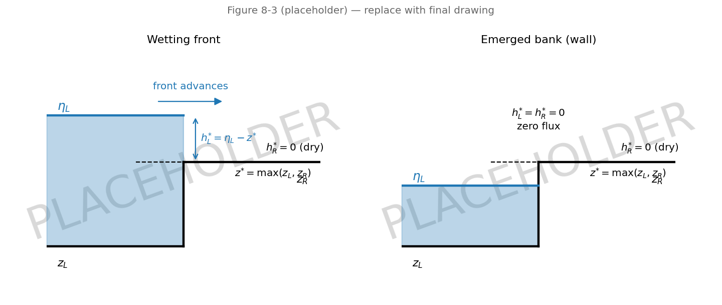
Figure 8-3 Hydrostatic reconstruction at a wet/dry front: an advancing front (left) and an emerged bank acting as a wall (right) (placeholder)
Implementation. The constants are kDryDepth, kDryArea and kEtaDeadband in src/engine/hydraulics/fv/FvKernels.hpp; the dry-bed signal speeds are openswmm::fv::kernels::waveSpeeds and the null face state is produced in openswmm::fv::ExplicitFvSolver::faceSide. Dry-cell zeroing is in openswmm::fv::ExplicitFvSolver::updateCells and openswmm::fv::ExplicitFvSolver::refreshDepths; compaction in openswmm::fv::ExplicitFvSolver::rebuildActiveLists (kRebuildInterval = 8); shoreline seeding in Router::initFv (src/engine/hydraulics/Routing.cpp).
The mesh and state are stored as structures of arrays over three index spaces, all fixed after initialization:
[0, n_cells) — per cell: a geometry index, the owning conduit row, length \(\Delta x\), mid-point bed elevation \(z_b\), the exact bed gradient \(dz/dx\), and the two bounding faces together with the side the cell occupies on each. State: area \(A\), discharge \(Q\), and the derived depth, free surface and velocity, refreshed after every update so faces read a consistent depth without re-inverting. A one-dimensional cell has exactly two faces, so the cell update is a fixed-width gather with no atomics and no scatter races — deterministic and identical across backends and thread counts.[0, n_faces) — per face: left and right cell indices (−1 marks a node on that side), the coupled node, the interface bed elevation, orientation signs relating each incident cell's axis to the face's positive direction, a flap-gate mask and a culvert marker. Scratch per face: mass and momentum flux, contact speed, the two Audusse corrections of (8-10), and the positivity scale.[0, n_nodes) — per node: invert, rim depth, ponded area, surcharge depth, kind (junction, virtual, storage, outfall), the fixed junction storage area, the flattened depth–volume table for storage units, and a CSR list of incident faces with a sign per face (+1 when a positive face flux enters the node). State: volume (the prognostic ledger), head, surface area and the overflow accumulators.Cells of one conduit are contiguous, so the conduit-to-cell map is a begin/count pair. Maximal runs of cells joined by interior faces form chains, stored as a CSR that spans virtual junctions; chains supply the ordered stencil for second-order reconstruction and one tridiagonal system per chain for implicit dispersion.
One global (untiered) substep executes the following sequence:
FV_STRUCTURE_COUPLING SUBSTEP (skipped on the first substep of a routing step, whose forcing the caller has just computed).FV_ORDER 2.Under FV_TIME_INTEGRATION RK2 steps 5–12 run twice at the same \(\Delta t\) and the two results are averaged (through volume at nodes). Under local time stepping the same face, cell and node passes are issued per tier from the macro-cycle schedule of §8.5.6: at base substep \(s\) of a cycle, faces of tiers up to \(j_f = \mathrm{ctz}(s)\) fire ( \(K - 1\) at \(s = 0\)) and volumes of tiers up to \(j_v = \mathrm{ctz}(s + 1)\) close, where \(\mathrm{ctz}\) counts trailing zeros — faces book \(\pm F\,\Delta t\) into per-volume accumulators in place of the direct divergence, and volumes drain their accumulators when they fire.
The scalar kernels — closure, reconstruction, Riemann flux, friction, Courant bound, positivity scale — are single-source inline functions over plain data. The same bodies compile for the CPU solver and, annotated with Kokkos function markers, for an accelerated device backend selected by FV_BACKEND (AUTO stays on the CPU below FV_MIN_PARALLEL_CELLS cells). Geometry closures are fixed-size structures of about 2 kB per distinct cross-section, so they can be copied into device memory without owning containers.
Implementation. Mesh and state layout are openswmm::fv::NetworkMeshData and openswmm::fv::NetworkStateData (src/engine/hydraulics/fv/NetworkMeshData.hpp), built by src/engine/hydraulics/fv/NetworkMeshBuilder.cpp. The substep pipeline is openswmm::fv::ExplicitFvSolver::takeSubstep and openswmm::fv::ExplicitFvSolver::advance; the macro cycle is openswmm::fv::ExplicitFvSolver::runMacroCycle with openswmm::fv::ExplicitFvSolver::fireFaces, openswmm::fv::ExplicitFvSolver::fireCells and openswmm::fv::ExplicitFvSolver::fireNodes, all in src/engine/hydraulics/fv/ExplicitFvSolver.cpp. The kernel bodies live in src/engine/hydraulics/fv/FvKernels.hpp behind the OPENSWMM_KERNEL_FN marker.
A node is where conduit control volumes meet. The end cell of each conduit exchanges with its node through a ghost state built from the node head, and that exchange goes through the same Riemann solver as an interior face. Wave reflection off the node, choking, supercritical approach flow and the surcharge transition are therefore resolved by the same shock-capturing machinery as the interior, rather than by a \(dQ/dH\) linearization.
What differs from node to node is where that head comes from. Three models are in use, chosen automatically from the node's own kind and connectivity — there is no user option:
| Model | Applies to | Storage | Head |
|---|---|---|---|
| Pass-through | a clean junction of degree 2 with nothing injected at it | none | not a state at all: the two end cells present their centred states directly to each other |
| Solved algebraic | every other storage-less junction with at least one conduit face | none | root of the instantaneous flux balance (8-31) |
| Bucket | storage units, junctions with no conduit face (a pump-only wet well), and junctions demoted by ponding | \(A_{s}\) or a curve | integrated volume ledger, §8.6.5 step 5 |
Clean means every incident face is a plain conduit face — no culvert inlet, no flap gate. A culvert or gate law is head- and direction-dependent and has to act against a solved node state, so it revokes both the direct splice and the reported reconstruction of §8.7. Outfalls are a fourth case and simpler than any of these: their stage is imposed every routing step, including FREE and NORMAL outfalls, whose depth setAllOutfallDepths computes from the conduit that feeds them. An outfall never integrates a ledger.
The ghost state is built directly from the node head \(H\) — for every node that has one, which is all of them but the pass-through case below. With \(z_f\) the conduit invert at the coupled face,
\[h_{g} = \max\left( 0,\ H - z_{f} \right), \qquad v_{g} = v_{int}, \qquad Q_{g} = A\left( h_{g} \right)\,v_{g}\] | (8-28) |
where \(v_{int}\) is the interior end cell's velocity expressed in the face frame — a transmissive momentum condition, sketched in Figure 8-4. A node standing below the face invert presents a dry ghost, so a perched pipe outlet drains as a free overfall. A closed conduit end with no node (a dead end) instead mirrors the interior state with reversed velocity, which returns exactly zero mass flux and leaves the interior its own hydrostatic pressure.
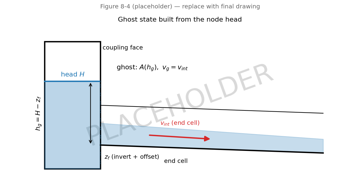
Figure 8-4 Node ghost-state construction at a coupling face (placeholder)
A plain junction has no storage. It is an interface, not a state: the water standing "in the manhole" is held by the incident end cells, which are real control volumes with their own depth. This mirrors the dynamic wave solver, where node_getSurfArea is exactly zero for a non-storage node and all working area belongs to the conduits — here, to the cells. The head is then the root of the instantaneous balance over the incident faces,
\[R(h) = \sum_{f} s_{f}F_{f}(h) + q_{lat} + q_{struct} + \frac{\text{carry}}{\Delta t} = 0\] | (8-31) |
with every face re-solved by the ghost-Riemann machinery (8-28) at each trial head, bracketed by geometric expansion and closed by a bracketed quasi-Newton step \(\delta h = R/\sum\sqrt{gAT}\). The remainder the iteration does not close is banked, not stored: it is carried to the next substep, and at a pass-through node it is disposed as volume into the incident cells, split evenly with zero momentum, because that is where an interface junction's water physically stands. The node volume the report shows for such a node is that carry ledger and nothing else.
Where a bucket ledger is integrated — storage units, structure-only junctions, ponding-demoted junctions — the storage relation is the engine's own: a linear reservoir of area \(A_{s} = V_{full}/y_{full}\) (MIN_SURFAREA unless the project overrode it) held fixed for the run, or the storage unit's own curve flattened to a monotone 129-sample depth–volume table. Two properties follow from \(A_{s}\) being constant, and both are load-bearing: \(V = A_{s}d\) is a genuine state relation, so re-seeding the ledger from the head between routing steps is exact rather than creating \((A_{s}^{new} - A_{s}^{old})d\) of water from nothing; and the volume the solver holds is the same function of depth the mass balance reports, so no water is stored where continuity cannot see it.
Why not give the node half of each connected link's volume? That is the dynamic wave convention, and it is deliberately not used here. In dynamic wave a conduit carries no depth state of its own at the node, so \(\sum \tfrac{1}{2}L\,T\) of surface area is how the node acquires any storage at all. Under finite volume the end cells already are control volumes holding exactly that water as explicit state, so adding a half-link area to the node books the same water twice. It was measured twice and rejected twice: tracking the live conduit top width — the obvious first guess — cost about 0.3 % of routing continuity on Example1, and the surviving MIN_SURFAREA-times-depth volume credit re-counted the cells' water at −0.005 % per junction on a 120-junction chain and was removed. The finite-volume analogue of the half-link volume is not a node term at all; it is the end cells, and the pass-through path already routes lateral inflow and residual carry into those cells, half to each side.
Mass is conserved exactly at a node. Momentum is intentionally not. At a general junction — several pipes at arbitrary angles, differing sections, a drop manhole — one-dimensional momentum conservation is ill-posed, because momentum is a vector and the pipe axes do not align. The standard stagnation-volume closure applies: velocity is zero in the node, pressure is hydrostatic, and all connected conduits share one piezometric head. This is the same conceptual model the dynamic wave solver uses, and like it, it is not an energy balance either — equating piezometric head discards the incoming velocity head, a dissipative closure appropriate to a chamber.
That dissipation has a measurable consequence, and it is the reason the pass-through model exists. Presenting a solved node head to two collinear cells splits one interior Riemann problem into two, and the split costs roughly a millimetre of head per junction. On a 199-junction subcritical chain that integrates into a 0.23 m backwater (SWASHES macdonald-long-sub, L1 depth error 0.228 → 0.0064 once the splice is used instead); with lateral inflow at every junction of a 400-conduit channel it reached an 18–25 % deep bias. A clean degree-2 junction therefore does not present a head at all — each of its two faces shows the far cell's full centred state, reproducing the single spliced face the pair stands in for. A lateral inflow does not revoke this, because a manhole pour carries no directed momentum: the inflow is diverted into the two incident cells, half each, as a zero-momentum area source. A structure flow or an unbled carry does revoke it, since both need a head the fluxes can respond to.
A bucket node's coupling to its faces is semi-implicit. Its storage area is typically the MIN_SURFAREA floor, which as an effective length \(A_{s}/T\) is a few feet against a conduit \(\Delta x\) of several hundred. Under explicit coupling it is therefore the manhole, rather than the pipe, that sets the stable substep for the whole model — which, before junctions became interfaces, was the whole network's substep. The semi-implicit coupling — always on; the explicit alternative was retired with FV_NODE_COUPLING — removes that by linearizing each coupling face's mass flux in the node head, using the characteristic relation \(\left| \partial Q/\partial H \right| = gA/c = \sqrt{g\,A\,T}\) at the ghost state:
\[\Delta H = \frac{\Delta t\left( \sum F + q_{lat} \right)}{A_{s} + \Delta t\sum\sqrt{g\,A\,T}}\] | (8-18) |
The resistance term is always positive — raising the head drives more out and lets less in, on either side of a face — so the denominator can only grow and the correction can only damp.
Conservation is preserved by construction. The correction is applied to the face flux itself, which is the single quantity both the cell update and the node update read, so whatever it does, the two sides of every face see the same number. Damping the node head directly instead — the obvious approach — would imply a volume change the incident cells never saw, trading exact mass conservation for stability. At equilibrium the correction is identically zero, since it is proportional to the node's net imbalance, so the two couplings agree on the steady state they reach.
The head correction is distributed over the incident faces through the same characteristic resistance,
\[\Delta Q_{f} = -\,s_{f}\,\sqrt{g\,A_{g}\,T_{g}}\ \Delta H\] | (8-29) |
where \(s_f\) is +1 when a positive face flux enters the node and −1 when it leaves, and \(A_g\), \(T_g\) are evaluated on the ghost state (8-28). §8.6.5 gives the complete update sequence, together with the optional Picard iteration of this correction, its optional extension to the adjacent end cells, and the node's time-step bound.
The semi-implicit coupling removes the node's stability limit but not its accuracy requirement: an under-resolved manhole is still under-resolved however stable it is. Local time stepping supplies the resolution cheaply, by giving the node its own fine tier while the conduit cells stay coarse. With FV_LTS NO there is nowhere to put the requirement but the global step, so the node's Courant limit is honoured there.
Where a connection really is two collinear pipes of identical section — the one case where one-dimensional momentum conservation is well posed — the model declares a virtual junction (see the [VIRTUAL_JUNCTIONS] section). Under finite-volume routing these are consumed at mesh construction: the two conduits' cell chains are concatenated and the junction becomes an ordinary interior face.
An inlet junction ([INLET_JUNCTIONS], Chapter 3 §3.3.10) is a virtual junction that also owns a street inlet and exchanges captured flow with a capture node at every step. Splicing it out would leave that transfer with no node to act on, so inlet junctions are not admitted under finite-volume routing: the input processor refuses them with error 619.
Nothing else is done, and nothing else is needed. Mass and momentum flux continuity across a virtual junction are then properties of the scheme rather than a special treatment, and a conduit split by a virtual junction reproduces the unsplit conduit cell for cell.
The one node-level quantity a virtual junction can still carry is a point lateral inflow (Chapter 3, §3.3.10). The node owns no face, so the inflow is divided equally between the two cells adjoining its spliced face and enters their mass equations as a zero-momentum source — the same treatment a clean degree-2 junction's lateral receives (§8.6.3) — and the node reports its through-flow plus the lateral as total inflow. A device backend that receives the per-node lateral must apply the same split; integrating it on the node would discard it.
Outfalls are stage boundaries: the head computed by the existing free/normal/fixed/tidal/time-series logic is imposed, and the ghost cell is built from it.
Pumps, orifices, weirs and outlets are evaluated by their existing structure equations and applied as source/sink pairs on the two node volumes. Under FV_STRUCTURE_COUPLING SUBSTEP (the default) they are re-evaluated at the top of every substep, together with the outfall stage, against the state the solver has actually reached — a routing step spans many substeps, across which a pump's wet-well depth and a weir's head difference move while a frozen discharge does not. ROUTING_STEP holds them at their start-of-step values instead.
Control rules are not re-evaluated at substep cadence; they run on the engine's own rule step, which is tuned for routing-step cadence. Only the head-dependent discharge of the structures those rules set is refreshed. A device backend cannot call the structure equations across the plugin boundary and clamps to ROUTING_STEP, saying so at open.
Culvert inlet control (§8.6.4) is applied inside the solver, as a cap on the flux crossing the culvert's upstream face, rather than by rewriting the link flow afterwards — the node ledger is booked from those fluxes, so a post-hoc rewrite would leave the reported flow and the continuity balance describing different runs.
A conduit or outfall flap gate masks the reverse flux at the conduit's boundary faces. The gate is a check valve, so a masked face behaves as a wall only while the flux would run the wrong way; closing it mirrors the interior state across the face, which returns exactly zero mass flux and leaves the interior its own hydrostatic pressure.
Lateral inflows enter at nodes exactly as assembled for any other routing method; at a virtual junction the inflow is split between the two spliced cells (§8.6.2). Distributed conduit losses — evaporation and seepage — enter the cell mass equation as \(q_L\) in (8-1).
A conduit carrying a culvert code in [XSECTIONS] marks its upstream boundary face at mesh construction, and the FHWA inlet-control curve for that code (the same unsubmerged/transition/submerged relations described in Chapter 7) is resolved to its coefficients at build time, so the solver evaluates the closure with no engine dependency. Whenever the computed mass flux at that face is directed into the culvert, the inlet-control discharge \(Q_{cap}\) is evaluated from the headwater depth at the node, compared per barrel exactly as the dynamic wave path compares it. If \(Q_{cap}\) is less than the Riemann flux, the face becomes a prescribed-discharge boundary and its flux is replaced by the physical flux at that discharge, evaluated on the upwind (node-side) reconstructed state:
\[\mathbf{F} = \begin{bmatrix} Q_{cap} \\ Q_{cap}^{2}/A_{up} + g\,I_{1,up} \end{bmatrix}\] | (8-30) |
Replacing the whole flux is required for self-consistency: scaling the Riemann momentum flux together with the mass flux strips the pressure term that resists the flow (measured as a 58 ft/s startup velocity spike), while scaling the mass flux alone leaves an unreduced momentum flux (151 ft/s). The cap acts on the face flux itself, before the node ledger is booked, so the reported flow and the continuity balance describe the same run. Conduits capped at any point in a routing step are flagged in the report's inlet-control column.
Implementation. openswmm::fv::ExplicitFvSolver::computeFaceFlux applies the cap through hydkernels::culvertInflow (src/engine/hydraulics/HydClosureKernels.hpp); the resolved curve is the culvert_curve member of openswmm::fv::FvGeometry, filled by src/engine/hydraulics/fv/NetworkMeshBuilder.cpp.
At the top of each routing step the solver re-derives every node's volume from the head the engine currently holds — so API writes, hot starts and stage updates take effect — and scatters the structure flows of §8.6.3 into a per-node net source \(q_{struct}\). With the junction area fixed for the run this re-seed is exact: it reproduces the volume the previous step ended with rather than perturbing it.
Each substep then advances every non-virtual node as follows. Steps 2 and 4 through 6 are the bucket path; a pass-through junction skips the node update entirely (its faces already carry the splice) and a solved algebraic junction replaces steps 2–6 with the root find (8-31) and its carry ledger.
FV_NODE_CELL_COUPLING once eliminated each end cell from a joint backward-Euler system with the node, so that the correction responded to the head difference between node and cell; it was superseded by the interface treatment above — a junction that holds no volume has nothing to couple to its end cells — as was FV_JUNCTION_MODEL. FV_NODE_PICARD iterated the correction of step 2, re-solving the incident faces at each provisional head; it corrected the mass fluxes only, leaving the momentum fluxes inconsistent with them — the same mass-only-correction defect the interface solve exists to avoid — and shipped with a recorded negative result (it never bought back the coarse step it was meant to). FV_NODE_COUPLING EXPLICIT and FV_NODE_DT NONE are retired on the same terms (§8.6.1 and the bound below); asking for any of the three retired behaviours is answered with a warning at open, while spelling out the former defaults is not.SURCHARGE_DEPTH above the rim, beyond which the excess volume is removed as flooding and the depth capped. This mirrors the dynamic wave solver's rule, so a model floods and ponds the same way under both solvers.The node's time-step bound. A bucket node behaves as an extra control volume of effective length \(A_{s}/T\), giving the bound
\[\Delta t \leq \alpha\,\frac{A_{s}/T}{\left\lvert v \right\rvert + c}\] | (8-32) |
evaluated over the node's wet incident end cells, and always armed. It is skipped for the nodes that have no volume state to protect — algebraic junctions, whose tier is instead pinned to their incident cells so that their faces fire together, and outfalls, whose head is imposed — which is why in practice it binds storage nodes only. Applying it to plain junctions was how a single MIN_SURFAREA bucket used to set a millisecond step for the whole network. The semi-implicit correction is unconditionally stable, so the bound controls accuracy rather than stability: when local time stepping is running, the bound is dropped from the global census and each node receives its own fine tier from (8-32), which supplies the resolution at low cost; when tiering cannot run (RK2, or transport), the bound is honoured in the global census. It is not optional: measured against the SWASHES analytic solutions under the earlier bucket junction model, dropping it was 24–134× faster and degraded the L1 depth error by factors of 3 to 49 on the frictional and transcritical cases (the FV_NODE_DT NONE switch that produced those numbers is retired; asking for it warns and is ignored).
Implementation. openswmm::fv::ExplicitFvSolver::relaxNodeFluxes and openswmm::fv::ExplicitFvSolver::relaxOneNode implement step 2; openswmm::fv::ExplicitFvSolver::updateNodes and openswmm::fv::ExplicitFvSolver::fireNodes carry the ledger on the global and tiered paths; openswmm::fv::ExplicitFvSolver::applyNodeCapacity implements step 6; the storage relation is openswmm::fv::ExplicitFvSolver::nodeVolumeFromDepth and openswmm::fv::ExplicitFvSolver::nodeDepthFromVolume with the slope openswmm::fv::ExplicitFvSolver::nodeStorageSlope; the bound (8-32) is openswmm::fv::ExplicitFvSolver::nodeStableDt. Options are declared in src/engine/hydraulics/fv/FvOptions.hpp.
The solver publishes per-link and per-node results at each routing step, so every existing report, output file and statistic works unchanged.
Link discharge is the length-weighted time mean over the routing step rather than an end-of-step sample: a routing step can span hundreds of substeps, and a sample aliases badly against them. Link depth and volume are instantaneous, as under dynamic wave routing. A virtual junction reports the state of the interior face that replaced it, and zero volume — it has none by construction.
Reported link depth is a water depth, truncated at the section's full height. Internally the solver's mean state above the crown is piezometric — depthOfArea of the slot-inclusive mean area — but the published depth is min(depthOfArea(A_mean), y_full), matching the dynamic-wave convention. The .out LINK_DEPTH column therefore never doubles as a head channel, and the Link Flow Summary's "Max/Full Depth" reads at most 1.00 for a closed conduit. The surcharge head remains fully visible where it belongs: in the node depths/heads (which are genuine piezometric state) and in the slot-storage accounting below. The truncation is publish-only — velocity, capacity, Froude number, surcharge hours, and the volume/slot ledgers are computed from the mean area or from saturating section geometry and are unaffected.
The Preissmann slot's water is genuine storage in the conservation ledger: link volume is \(\sum A\,\Delta x\) over the slot-inclusive conserved area, with no clamp, and it feeds Final Stored Volume and SYS_STORAGE at full weight. Because plain junctions report zero storage under FV (their water stands in the incident cells), the slot is the only place surcharge storage can be booked — so on a pressurized system a material share of reported storage can stand in the slot. The engine separates that share out rather than leaving it folded in:
links.slot_volume — per link, \(\sum \max(0,\,A - A_{crown})\,\Delta x\), always a subset of the link volume, zero below the crown and zero under dynamic-wave routing. C API: swmm_link_get_slot_volume.swmm_link_get_stat_slot_share (run-level) and swmm_link_get_stat_peak_slot_share (peak, 0..1).OPENSWMM_FV_SLOT_TRACE=1 — one CSV row per routing step on stdout (SLOT_TRACE,t,slot_ft3,stored_ft3,share), for plotting the slot share through a transient.The FV Solver Statistics block attributes the time step alongside: four "dt Argmin" rows give the fraction of CFL censuses whose binding element was a pressurized cell (at or above the crown), a taper-band cell, a free-surface cell, or a node bound. On a pressurized system the pressurized rows dominating is the measured statement that FV_SLOT_CELERITY — not the free-surface dynamics — is setting the run's cost.
Two properties of the slot worth reading off these instruments rather than assuming: the slot share of storage scales as \(1/c^{2}\) in the celerity, and the steady full-bore head loss depends on the celerity — the slot absorbs part of the friction grade — converging on the Manning value from below as the slot narrows. A low celerity therefore understates both pressurization and head loss at once; the 5 % width cap (§8.4.1) bounds the damage but does not remove it, and WARNING 108 reports when the cap has silently overridden the requested celerity (every request below the cap-implied celerity produces byte-identical geometry).
Node stage is reconstructed from the incident cells, not read off the solver's head. For a storage-less clean junction of any degree — the publish rule is the clean test of §8.6.1 without its degree-2 restriction, since reconstructing a reported stage needs no splice — the published head is
\[H_{pub} = \max_{f\ \in\ \text{wet},\ z_{f} \leq H} \left[\ \min\left(z_{b,c(f)},\, z_{f}\right) + h_{c(f)}\ \right]\] | (8-33) |
taken over the node's wet incident faces. A dry neighbour's vote would be bare ground, and a face perched above the node's own surface is discharging as a free overfall — its stage describes the pipe's offset, not the node — so neither votes; with no wet vote at all the solver's head stands. This is the same reconstruction the virtual-junction rule uses, which is what keeps a junction and a virtual junction from stepping against each other in a plotted HGL.
The reason is that the solver's own head for a solved algebraic junction carries a half-cell datum offset of order \(S_{0}\Delta x/2\) against the face stage, which appears in a profile plot as a step at the manhole. It is a reporting term, not a routing one: it falls first-order under mesh refinement, it survives on nodes with no lateral inflow at all, and correcting it leaves the routed solution bit-identical. Measured on Example1 at FV_MIN_CELLS 1, where the comparison against the adjacent cell is exact, the largest excess over the adjacent conduit surface falls from 0.91 ft to below 0.001 ft. Reporting is deliberately the only place this correction is applied: solver-internal heads double as ghost boundary states under local time stepping, and changing the in-solver estimator turned a 0.007 cfs lake-at-rest residual into a 70.9 cfs standing oscillation.
Bucket nodes, culvert headwaters, gated nodes and nodes carrying a structure flow are excluded and publish the head the solver holds, which for them is a genuine state.
When the solver carries advected species, the species flux is the same mass flux the water used, upwinded on the contact speed (8-12):
\[F_{\varphi} = F_{mass}\varphi_{L} \ \text{ if } S^{*} \geq 0, \qquad F_{\varphi} = F_{mass}\varphi_{R} \ \text{ if } S^{*} < 0\] | (8-17) |
Flux consistency is essential here. Computing the species flux from a separately evaluated velocity — the usual result of bolting transport onto a hydraulic solver — decouples solute mass from water mass and produces spurious concentration extrema. Reusing \(F_{mass}\) guarantees exact solute conservation, and that a uniform concentration field stays uniform under any flow, including reversal and wetting and drying.
FV_SCALAR_SCHEME selects the reconstruction: first-order UPWIND, MUSCL (the default), or QUICKEST_ULTIMATE (Leonard, 1979, 1991), which is third order where its two-cell upstream stencil exists and degrades to MUSCL where it does not. The higher-order fluxes are limited by the flux-corrected transport construction of Zalesak (1979), which enforces the discrete maximum principle — no new extrema, no negative concentrations — while preserving conservation exactly. Clipping the updated concentration instead would enforce the bound but destroy conservation.
Longitudinal dispersion (FV_DISPERSION) is treated implicitly, one tridiagonal solve per cell chain. The explicit stability limit for a parabolic term is \(\Delta t \le \Delta x^{2}/2D_{L}\), which at fine \(\Delta x\) is far more restrictive than the Courant condition; the implicit treatment removes it entirely.
All knobs are [OPTIONS] keys. They are accepted and inert under any other routing model, so switching FLOW_ROUTING never invalidates a file.
| Key | Default | Meaning |
|---|---|---|
FV_CELL_LENGTH | 0 | Target \(\Delta x\) in project length units. 0 means no length target; each conduit gets FV_MIN_CELLS cells. |
FV_MIN_CELLS | 4 | Floor on cells per conduit. Applies with or without a FV_CELL_LENGTH target. |
FV_CFL | 0.5 | Courant number \(\alpha\) in (8-14). |
FV_RIEMANN | HLLC | Species flux: HLLC resolves the contact wave, HLL averages it. No effect on hydraulics. |
FV_ORDER | 1 | 1 or 2. Second order is MUSCL on \((\eta, v)\) with the guard of §8.5.6. |
FV_LIMITER | MINMOD | MINMOD, VANLEER or SUPERBEE, with FV_ORDER 2. |
FV_SCALAR_SCHEME | MUSCL | UPWIND, MUSCL or QUICKEST_ULTIMATE. |
FV_TIME_INTEGRATION | EULER | EULER or RK2 (Heun, SSP). RK2 disables local time stepping. |
FV_SLOT_CELERITY | 100 | Pressurized wave celerity in project length units per second; sets the slot width via (8-5) and doubles as the TPA acoustic celerity \(a\) under FV_PRESSURE_CLOSURE TPA (§8.4.5) — the same physical dial either way. Slot storage share scales as 1/c²; values below the cap-implied celerity (≈ 22.5·√D ft/s for a circular pipe) are inert — WARNING 108 reports the override. Slot storage is itemized by the §8.7.1 diagnostics. With FV_PRESSURIZED_IMPLICIT YES the celerity leaves the time-step law entirely (§8.4.4) and becomes a pure accuracy dial. |
FV_PRESSURE_CLOSURE | SLOT | Experimental — SLOT or TPA. TPA selects the two-component pressure approach of §8.4.5: sub-atmospheric full-pipe flow behind a per-cell air-pathway regime flag. SLOT (the default) is bit-identical to the closure of §8.4.1–§8.4.2. Pair with REPORT_SIGNED_HEADS YES to see sub-atmospheric heads in the .out file. |
FV_PRESSURIZED_IMPLICIT | NO | Experimental — subject to slot program R2b; surfaced in the GUI as an experimental checkbox. Integrate the slot's acoustic pair implicitly on the pressurized subset (§8.4.4): full-bore head loss becomes slot-width invariant and pressurized reaches run at the advective time-step bound. CPU solver only; local time stepping stands down while the solve engages; a run that never pressurizes is bit-identical either way. Composes with FV_PRESSURE_CLOSURE TPA under the rules of §8.4.5. |
FV_DISPERSION | 0 | Longitudinal dispersion coefficient. 0 disables the parabolic term. Accepted but inert until finite-volume transport is connected (§8.8); a non-zero value warns at open. |
FV_STRUCTURE_COUPLING | SUBSTEP | Cadence at which structure flows and outfall stages are refreshed: every substep, or once per routing step. A device backend clamps to ROUTING_STEP. |
FV_NODE_CELL_COUPLING | — | Retired. Accepted and ignored so existing projects still parse; junctions are always interfaces (§8.6.1). FV_JUNCTION_MODEL is retired on the same terms. |
FV_NODE_COUPLING, FV_NODE_DT, FV_NODE_PICARD | — | Retired 2026-08-29. Storage-node coupling is always semi-implicit (§8.6.1), the node bound (8-32) is always armed (§8.6.5), and the correction is always a single sweep — each the former default. Accepted so existing projects still parse; a value asking for the retired behaviour (EXPLICIT, NONE, sweeps above 1) warns at open and is ignored. |
FV_COMPACTION | YES | Skip dry, inactive parts of the network. Results-transparent. |
FV_LTS | YES | Local time stepping (§8.5.6). NO forces one global substep size. |
FV_LTS_MAX_TIERS | 6 | Cap on the tier spread; 6 allows 64×. |
FV_CFL_CENSUS_INTERVAL | 1 | Substeps between full Courant censuses. 1 recomputes every substep. |
FV_BACKEND | AUTO | CPU, AUTO, OMP, CUDA, HIP or SYCL. |
FV_MIN_PARALLEL_CELLS | 20000 | Mesh size below which AUTO stays on the CPU. |
Three keys without the FV_ prefix also affect finite-volume runs and are shared with the dynamic wave solver: UNSTEADY_FRICTION and UF_K3 (§8.5.4), and REPORT_SIGNED_HEADS (§8.4.5), which puts the true signed piezometric head in the .out HEAD field for both solvers (default NO keeps legacy bit-parity; DEPTH stays floored either way).
Measured on 2026-08-20 against commit 962fd48c, on the EPA reference site drainage model (Example1.inp, 30 h, 5 s routing step) and on generated uniform and graded reaches. Reproduce with tests/benchmarks/scripts/fv_perf_baseline.py; the full tables, the per-phase split and the .out hashes are in plans/FV1D_PERF_BASELINE_2026-08-20.md.
| Dynamic wave | FV, 1 cell | FV, default (4 cells) | |
|---|---|---|---|
| Routing continuity error | 0.026 % | 0.000 % | −0.000 % |
| Wall-clock, relative | 1× | 5.3× | 14.9× |
| Substeps per routing step | — | 1.03 | 2.05 |
The same comparison across network size, on uniform and graded reaches of 50 / 500 / 2000 conduits, at the default mesh:
| 50 | 500 | 2000 | |
|---|---|---|---|
| uniform reach, × dynamic wave | 11.3 | 17.3 | 17.5 |
| graded reach, × dynamic wave | 15.6 | 33.5 | 29.2 |
| routing continuity, finite volume | 0.000 % | −0.000 % | −0.000 % |
| routing continuity, dynamic wave | −1.30 / −0.59 % | −0.51 / −0.80 % | −0.51 / −0.64 % |
Three observations follow.
Conservation is delivered, and is independent of resolution. The finite-volume solver closes continuity exactly on every deck and every mesh above, where the implicit solver does not — and the gap is widest on the plain reaches, where dynamic wave loses 0.5 % to 1.3 % of volume. That is the property the conservation form guarantees.
Accuracy requires a resolved mesh. An unresolved mesh is not a drop-in substitute for dynamic wave analysis. The mechanism is the artificial bed step of §8.3 rather than numerical diffusion, so second-order reconstruction does not remove it.
It costs several times more, and the multiple grows with the network. At one cell per conduit — the same element count dynamic wave carries — the explicit method runs about five times its wall clock on the reference model, and the default mesh roughly triples that again. On uniform reaches the ratio rises from 11× at 50 conduits to 17× at 2000, so the cost should not be expected to amortize on larger models. Select the method for its conservation and shock-capturing properties, not for speed.
Note that the earlier editions of this section reported ratios of 39× to 252× across the same reach sizes. Those numbers were measured on the bucket-junction solver that 265eb727 (2026-08-11) replaced with algebraic junctions, and they no longer describe this solver; the table above supersedes them.
Practical guidance:
FV_CELL_LENGTH.SURCHARGE_METHOD SLOT with a tightened HEAD_TOLERANCE addresses most of it at no cost, and virtual junctions remove the storage error at genuine grade breaks.FV_PRESSURE_CLOSURE TPA (§8.4.5) lifts this, down to the column-separation bound of about −30 ft of head; air-phase effects remain out of scope under either closure.Audusse, E., Bouchut, F., Bristeau, M.-O., Klein, R., and Perthame, B. (2004). "A fast and stable well-balanced scheme with hydrostatic reconstruction for shallow water flows." SIAM Journal on Scientific Computing, 25(6), 2050–2065.
Davis, S. F. (1988). "Simplified second-order Godunov-type methods." SIAM Journal on Scientific and Statistical Computing, 9(3), 445–473.
Harten, A., Lax, P. D., and van Leer, B. (1983). "On upstream differencing and Godunov-type schemes for hyperbolic conservation laws." SIAM Review, 25(1), 35–61.
Hou, T. Y., and LeFloch, P. G. (1994). "Why nonconservative schemes converge to wrong solutions: error analysis." Mathematics of Computation, 62(206), 497–530.
Leonard, B. P. (1979). "A stable and accurate convective modelling procedure based on quadratic upstream interpolation." Computer Methods in Applied Mechanics and Engineering, 19(1), 59–98.
Pinto, S. I. G., Vasconcelos, J. G., and Soares, A. K. (2025). "Unsteady friction in mixed-flow models based on the Saint-Venant equations." Journal of Hydraulic Engineering, 152(1), 04025046.
Vasconcelos, J. G., Wright, S. J., and Roe, P. L. (2006). "Improved simulation of flow regime transition in sewers: two-component pressure approach." Journal of Hydraulic Engineering, 132(6), 553–562.
Vasconcelos, J. G., Wright, S. J., and Roe, P. L. (2009). "Numerical oscillations in pipe-filling bore predictions by shock-capturing models." Journal of Hydraulic Engineering, 135(4), 296–305.
Vítkovský, J. P., Lambert, M. F., Simpson, A. R., and Bergant, A. (2000). "Advances in unsteady friction modelling in transient pipe flow." Proc., 8th Int. Conf. on Pressure Surges, BHR Group, The Hague, Netherlands.
Leonard, B. P. (1991). "The ULTIMATE conservative difference scheme applied to unsteady one-dimensional advection." Computer Methods in Applied Mechanics and Engineering, 88(1), 17–74.
Toro, E. F. (2001). Shock-Capturing Methods for Free-Surface Shallow Flows. Wiley, Chichester.
Zalesak, S. T. (1979). "Fully multidimensional flux-corrected transport algorithms for fluids." Journal of Computational Physics, 31(3), 335–362.
 1.13.2