|
OpenSWMM Engine
6.0.0-alpha.4
Data-oriented, plugin-extensible SWMM Engine (6.0.0-alpha.4)
|
|
OpenSWMM Engine
6.0.0-alpha.4
Data-oriented, plugin-extensible SWMM Engine (6.0.0-alpha.4)
|
______________________________________________________________________________
SWMM can model evaporation and seepage losses from conduits as a uniformly distributed lateral outflow along the length of the conduit. The following paragraphs explain how user-supplied evaporation and seepage rates per unit area are converted into a distributed loss per unit length for a conduit and how this loss rate is factored into the solution of the governing equations for both dynamic and kinematic wave modeling.
Distributed Uniform Evaporation Rate
SWMM can use time varying evaporation data from several different types of external sources. These include historical daily values from the National Weather Service, values computed from an historical record of daily temperatures, user-supplied monthly average values or a user-supplied hourly time series. The details are described in Volume I (Hydrology) of this reference manual. These data express the potential evaporation rate over the entire study area as a volumetric loss per unit of area per unit of time, which SWMM converts to internal units of cfs/ft2. The following expression converts the rate per unit area into a rate per unit length of channel (only open channels can evaporate) over the time period t to t+∆t:
\[q_{E} = e_{t}W\left( \overline{\overline{Y}} \right)\]
(7-1)
where \(q_{E}\) = uniformly distributed evaporation rate along a channel (cfs/ft) \(e_{t}\) = potential evaporation rate per unit area over the current time period (cfs/ft2) \(\overline{\overline{Y}}\) = average depth of flow in the channel over the current time period (ft) \(*W(Y)*\) = width of water surface at depth of flow Y (ft).
The program automatically extracts the appropriate rate et from the evaporation data source for the current time period being analyzed. The water surface width W is computed using the procedures described in Chapter 5 for a particular channel's cross sectional shape.
The average depth of flow in the channel is computed differently depending on the hydraulic modeling procedure used. For kinematic wave modeling,
\[\overline{\overline{Y}} = \frac{\left( {Y(A}_{1}^{t}) + {Y(A}_{2}^{t} \right))}{2}\]
(7-2)
where \(A_{1}^{t}\) is the flow area at the upstream end of the channel previously computed for time t, \(A_{2}^{t}\) is the same at the downstream end of the channel, and Y(A) is the flow depth associated with flow area A . The latter function is evaluated using the procedures described in Chapter 5.
For dynamic wave modeling the average channel depth is computed as:
\[\overline{\overline{Y}} = \frac{\left( {\overline{Y}}^{t} + {\overline{Y}}^{t + \mathrm{\Delta}t} \right)}{2}\]
(7-3)
where \(\overline{Y} = \frac{\left( Y_{1} + Y_{2} \right)}{2}\). The *Y1* and *Y2* values for \({\overline{Y}}^{t + \mathrm{\Delta}t}\) are evaluated with Equation 3-16 for the most recently computed nodal head solution Hlast in the iterative procedure used to solve the dynamic wave equations. Thus \(\overline{\overline{Y}}\) and therefore qE can change as the dynamic wave iterations unfold within a time step.
Distributed Uniform Seepage Rate
The seepage loss from a conduit could be due to infiltration into the soil beneath an unlined or natural channel or result from a leaking or perforated pipe. In theory the rate would depend upon such factors as the flow depth in the conduit, the hydraulic conductivity of the surrounding soil, the variation in moisture content of this soil and the depth to groundwater. Rather than try to rigorously model the dynamics of soil infiltration beneath the seeping conduit SWMM uses a user-supplied constant seepage rate per unit area that can be different for each conduit. At any given time period this rate is converted to a uniformly distributed rate per length of conduit as follows:
\[q_{S} = sf_{c}W(\overline{\overline{Y}})\]
(7-4)
where
| Symbol | = | Description | Units |
|---|---|---|---|
\[q_{S}\] | = | uniformly distributed seepage rate per length of conduit | cfs/ft |
| s | = | user-supplied seepage rate per unit area for the conduit | cfs/ft2 |
| fc | = | monthly climate adjustment factor for the current time step | dimensionless |
\[\overline{\overline{Y}}\] | = | average depth of flow in the conduit over the current time period | ft |
The monthly climate adjustment factors are a set of 12 user-supplied constants that apply to the study area as a whole. They allow the intensity of infiltration-based processes to vary on a seasonal basis. The average flow depth is computed using Equation 7-2 or 7-3, depending on the choice of flow routing method.
Equation 7-4 assumes that seepage occurs only in the vertical direction so that the area over which it takes place is limited by the largest horizontal extent of the flow cross section. Thus the average depth of flow \(\overline{\overline{Y}}\) is limited by the depth at which the cross section width is a maximum. Table 7-1 lists the depth at maximum width, as a fraction of full conduit depth, for several different cross section shapes recognized by SWMM. For other shapes not listed the depth at maximum width is as follows:
Table 7‑1 Relative depth at maximum width for select cross section shapes
| Shape | Relative Depth | Shape | Relative Depth |
|---|---|---|---|
| Circular | 0.50 | Horseshoe | 0.50 |
| Ellipsoid | 0.48 | Catenary | 0.25 |
| Arch | 0.28 | Gothic | 0.45 |
| Basket Handle | 0.20 | Semi-Circular | 0.15 |
| Egg | 0.64 | Semi-Elliptical | 0.15 |
Total Uniform Loss Rate
The total uniform outflow rate along a conduit qL is the sum of the evaporative and seepage loss rates:
\[q_{L} = q_{E} + q_{S}\]
(7-5)
Over any given time step ∆t the total volume lost to this outflow cannot exceed the average volume contained in the conduit:
\[q_{L}L\mathrm{\Delta}t \leq \overline{\overline{A}}L\]
(7-6)
where \(\overline{\overline{A}}\) is the average flow area over the time step and L is the conduit length. Thus
\[q_{L} = \min\left( q_{L},\frac{\overline{\overline{A}}}{\mathrm{\Delta}t} \right)\]
(7-7)
For kinematic wave analysis the average flow area over the time step from t to t+∆t is:
\[\overline{\overline{A}} = \frac{\left( A_{1}^{t} + A_{2}^{t} \right)}{2}\]
(7-8)
where \(A_{1}^{t}\) is the flow area at the upstream end of the conduit computed for time t and \(A_{2}^{t}\) is the same at the downstream end of the conduit. For dynamic wave analysis:
\[\overline{\overline{A}} = \frac{\left( {\overline{A}}^{t} + {\overline{A}}^{t + \mathrm{\Delta}t} \right)}{2}\]
(7-9)
where \({\overline{A}}^{t} = \frac{\left( A\left( Y_{1} \right) + A\left( Y_{2} \right) \right)}{2}\) for *Y1* and *Y2* computed at time t, with a similar expression used for \({\overline{A}}^{t + \mathrm{\Delta}t}\). In the latter case the flow depths Y are computed using the most recently computed nodal heads (see Equation 3-16) as the iterative dynamic wave solution unfolds.
An additional constraint on qL is that it cannot be greater than the inflow rate \(Q_{1}^{t + \Delta t}\) to the conduit under kinematic wave analysis or the last computed flow Qlast under dynamic wave analysis.
Dynamic Wave Modifications
For dynamic wave analysis, including a uniform loss rate adds an additional term *∆Qlateral* to Equation 3-14 used to update a conduit's flow rate over a time step. The revised equation is:
\[Q_{t + \Delta t} = \frac{Q_{t} + {\mathrm{\Delta}Q}_{inertia} + {\mathrm{\Delta}Q}_{pressure} + \mathrm{\Delta}Q_{lateral}}{1 + {\mathrm{\Delta}Q}_{friction}}\]
(7-10)
where \(\mathrm{\Delta}Q_{lateral} = 2.5\overline{U}q_{L}\) and all other ∆Q terms were defined previously in Section 3.2. See the sidebar below for the derivation of this modified equation.
Computing Geometry Table Entries for Irregular Cross Sections
To find the k-th entry in an irregular cross section's geometry tables first initialize the following:
Flow depth: \(Y = k \cdot Y_{full}/50\)
Table entries for index k: \(A_{tbl}[k] = 0\), \(W_{tbl}[k] = 0\), \(R_{tbl}[k] = 0\)
Compound segment area: \(A_{sum} = 0\)
Compound wetted perimeter: \(P_{sum} = 0\)
Total flow conductance: \(K = 0\)
Transect station index: \(i = 1\)
- Select the cross section segment between transect stations at \(x_{i-1}\) and \(x_i\).
- If the flow depth is below the channel bottom ( \(Y < \min(y_{i-1}, y_i)\)) go to step 10.
- Compute the width \(w\) and wetted perimeter \(p\) of the full segment: \(w = x_i - x_{i-1}\) \(p = \sqrt{w^2 + (\Delta y)^2}\) where \(\Delta y = |y_i - y_{i-1}|\)
- If the segment is completely submerged ( \(Y > \max(y_{i-1}, y_i)\)) compute its area \(a\) as: \(a = w(Y - (y_{i-1} + y_i)/2)\) Otherwise let \(\alpha = (Y - \min(y_{i-1}, y_i))/\Delta y\) and set \(a = \alpha^2 w \Delta y/2\).
- Adjust the width and wetted perimeter for partial submergence: \(w = \alpha w\); \(p = \alpha p\)
- Update the table entries for area and top width: \(A_{tbl}[k] = A_{tbl}[k] + a\); \(W_{tbl}[k] = W_{tbl}[k] + w\)
- Update the area and wetted perimeter of the current compound segment: \(A_{sum} = A_{sum} + a\); \(P_{sum} = P_{sum} + p\)
- Let \(n_i\) be the roughness coefficient between stations \(i-1\) and \(i\). If station \(i\) marks the end of a compound segment ( \(y_i > Y\) or \(n_i \neq n_{i+1}\)) then update the total conductance: \(K = K + (1.486/n_i) A_{sum} (A_{sum}/P_{sum})^{2/3}\) and begin a new compound segment by setting \(A_{sum}\) and \(P_{sum}\) to 0.
- If more transect stations remain, increment the station index, \(i = i + 1\) and go to Step 2.
- Compute the hydraulic radius table entry:
\(R_{tbl}[k] = ((n_C K)/(1.486 A_{tbl}[k]))^{3/2}\) where \(n_C\) is the main channel roughness.
Another modification needed when including a uniform loss rate is to add qLL (the total flow lost over the length of the conduit) to the total outflow from the upstream node of a conduit with positive flow or add it to the total inflow of the downstream node of a conduit with negative flow. This modifies the \(\sum_{}^{}Q^{t + \mathrm{\Delta}t}\) term (the net inflow minus outflow to a node) in Equation 3-15a which is used to update nodal heads.
Kinematic Wave Modifications
For kinematic wave analysis, adding a uniform loss term modifies the original continuity equation 4-1 as follows:
\[\frac{\partial A}{\partial t} + \frac{\partial Q}{\partial x} + q_{L} = 0\]
(7-11)
Carrying the qL term over into the original finite difference form of this equation (Equation 4-7) produces:
\[\frac{(1 - \theta)\left( A_{1}^{t + \Delta t} - A_{1}^{t} \right) + \theta\left( A_{2}^{t + \Delta t} - A_{2}^{t} \right)}{\Delta t} + \frac{(1 - \phi)\left( Q_{2}^{t} - Q_{1}^{t} \right) + \phi\left( Q_{2}^{t + \Delta t} - Q_{1}^{t + \Delta t} \right)}{L} + q_{L} = 0\]
(7-12)
where all notation was defined previously in Section 4.2. After substituting the Manning equation \(Q = \beta\Psi(A)\) into this expression the same non-linear equation for \(A_{2}^{t + \Delta t}\) results as before (equation 4-8):
\[\beta\Psi\left( A_{2}^{t + \Delta t} \right) + C1A_{2}^{t + \Delta t} + C2 = 0\]
(7-13)
with C1 given by Equation 4-9 and C2 by Equation 4-10 but with the additional term \(q_{L}\frac{L}{\phi}\) added to it.
An open storage unit can evaporate water from its top surface and, if unlined, can have a seepage loss due to water infiltrating into the soil beneath its bottom and sloped sides. SWMM represents each of these losses as a flow rate per unit area of surface exposed. The exposed surface area (top for evaporation, bottom and sides for seepage) is computed based on the storage unit's water depth at the start of each computational time step. The combined total loss rate (in cfs) from both processes is then subtracted from the net inflow to the storage unit so that its new water depth at the end of the time step can be computed.
Evaporation Loss
The evaporation loss rate from the surface of a storage unit during a time period is based on the surface area in the unit at the start of the time period using the following equation:
\[Q_{EN} = e_{t}f_{E}A_{SN}\left( Y^{t} \right)\]
(7-14)where
\(Q_{EN}\) = evaporation loss rate from a storage unit node (cfs)
t = starting time for the current computational time period (sec)
\(e_{t}\) = potential evaporation rate per unit area at time t (cfs/ft2)
fE = fraction of evaporation rate realized
Yt = depth of stored water at time t (ft)
*ASN(Y)* = storage unit surface area at water depth Y (ft).
The potential evaporation rate et is the same quantity discussed in the previous section on conduit evaporation and is automatically retrieved from a study area's evaporation data source as the simulation unfolds over time. The fraction of this rate realized, fE, is a user-supplied value for each storage unit that allows the rate to be adjusted for specific local conditions. It would normally be 1.0 but could be 0 if the storage unit has a roof over it. The depth of stored water *Ytis the difference between the water surface elevation *Ht at time t and the storage unit's invert elevation E. The A(Y) function represents the user-supplied curve of surface area versus depth as described in Section 5.4.
Seepage Loss
The seepage loss from a storage unit is modeled as infiltration of ponded water into the native soil beneath the unit. The Green-Ampt soil infiltration method is used to compute the rate of seepage per unit area over time. Its fundamental formula is:
\[q_{SN} = K_{S}f_{C}\left\lbrack 1 + \frac{\left( \psi_{S} + d \right)\theta_{d}}{F} \right\rbrack\]
(7-15)
where
*qSN* = seepage rate per unit area from the storage unit node (cfs/ft2)
KS = soil saturated hydraulic conductivity (ft/sec)
fC = monthly climate adjustment factor for the current time step (dimensionless)
d = depth of stored water above the area undergoing seepage (ft)
\(\psi_{S}\) = soil capillary suction head (ft)
*θd* = soil moisture deficit (dimensionless)
F = cumulative depth of infiltrated water (ft).
The monthly seepage adjustment factor is the same user-supplied set of multipliers used for conduit seepage described previously for equation 7-4. KS, ψS, and the initial value of θd are all parameters associated with the Green-Ampt model. Both θd and F are modified by the model over time. Equation 7-15 makes the seepage rate dependent on the ratio of stored water depth to cumulative infiltrated depth, both of which will vary over time
The details of SWMM's implementation of the Green-Ampt infiltration model are covered in Chapter 4 of Volume I (Hydrology) of this manual. The only difference when using it for a storage unit is that the quantity \(\psi_{s}\) in the original formulation is replaced with \(\psi_{s} + d\). Volume I also provides guidance on selecting values of KS, \(\psi_{s}\), and an initial θd based on soil type. If either \(\psi_{s}\) or θd are 0 then SWMM assumes a constant seepage rate equal to KS that is independent of storage depth. If KS is 0 then no seepage occurs.
The depth of water to use in the Green-Ampt formula will vary across the top surface of a storage unit if it has sloped sides as shown in Figure 7-1. SWMM accounts for this by applying the Green-Ampt infiltration method independently to two separate seepage areas – one for water in contact with the flat bottom portion of the unit and a second for water in contact with the sloped sides. The total seepage loss rate *QSN* (in cfs) can be expressed as:
\[Q_{SN} = q_{btm}\left( d_{btm} \right)A_{btm} + q_{side}\left( d_{side} \right)A_{side}\]
(7-16)
where:
*dbtm* = depth of stored water above bottom of unit (ft)
*qbtm* = Green-Ampt infiltration rate based on *d = dbtm* (cfs/ft2)
A*btm = surface area over which bottom seepage occurs (ft2)
*dside* = average depth of stored water above sloped sides of unit (ft)
*qside* = Green-Ampt infiltration rate based on *d = dside* (cfs/ft2)
*Aside* = surface area of sloped sides over which seepage occurs (ft2).
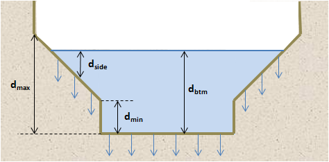
Figure 7‑1 Depths used for computing seepage in storage units
As noted previously, the depth above the bottom of the storage unit (*dbtm*) is \(Y^{t} = H^{t} - E\). The bottom surface area is found from the unit's storage curve at a depth of 0 (see Section 5.4 for a discussion of storage curves). The average depth above the sloped sides is computed as:
| Condition | Value | Equation |
|---|---|---|
| for \(Y^{t} < d_{\min}\) | \(0\) | (7-17) |
| for \(d_{\min} \leq Y^{t} \leq d_{\max}\) | \(\frac{\left( Y^{t} - d_{\min} \right)}{2}\) | |
| for \(Y^{t} > d_{\max}\) | \(Y^{t} - \frac{\left( d_{\max} - d_{\min} \right)}{2}\) |
where *dmin* is the storage depth where the sloped sides begin and *dmax* is the depth where it ends (see Figure 7-1). Both of these depths can be found from the storage unit's storage curve. The effective area over which vertical seepage through the sloped sides occurs is computed as:
\[A_{side} = min\left\{ A\left( Y^{t} \right),\ A\left( d_{\max} \right) \right\} - A_{btm}\]
(7-18)Total Storage Loss
The total loss rate from a storage unit node, *QLN* (in cfs), over a given time step is
\[Q_{LN} = Q_{EN} + Q_{SN}\]
(7-19)*QLN* is not allowed exceed the volume of water in storage at the start of the current time step:
\[Q_{LN} = min\left\{ Q_{LN},\frac{V_{N}\left( Y^{t} \right)}{\mathrm{\Delta}t} \right\}\]
(7-20)
where VN(Y) is the storage unit's volume at depth Y (see section 5.4 for how it is computed) and ∆t is the size of the current time step.
For a given storage node, QLN is computed once at the start of the current time step based on the known stored water level. For dynamic wave analysis it is subtracted from the \(\sum_{}^{}Q^{t + \mathrm{\Delta}t}\) term of Equation 3-15a (i.e., is treated as a nodal outflow) each time the node's head is updated at step 4 of the solution procedure described in Section 3.2. For kinematic wave analysis, after all link flows have been found, QLN is added to the node's total outflow at the end of the time step (see Equation 4-18) which is used to update the node's volume and subsequently its hydraulic head (see Section 4.3.5).
Energy losses caused by rapid changes in magnitude or direction of velocity are called minor or local losses. They can occur at bends, contractions, or enlargements in conduit geometry and also be associated with flows entering a conduit from a larger water body or flows exiting a conduit to a larger water body. Table 7-2 lists the types of minor losses most frequently considered in stormwater conveyance networks.
A minor loss is represented as the product of a loss coefficient and the local velocity head for a specific location i along a conduit:
\[\mathrm{\Delta}H_{L} = K_{m,i}\frac{U_{i}^{2}}{2g}\]
(7-21)
where \(\mathrm{\Delta}H_{L}\) is the minor head loss (ft), Km,i is a loss coefficient, and Ui is flow velocity (ft/sec). The location index i is 1 for an entrance loss based on the conduit's upstream velocity, 2 for an exit loss based on its downstream velocity, or 3 for an average loss based on its average velocity.
Minor losses can be included in the St. Venant momentum equation for a conduit by treating them as a loss per unit length, hL, in the same way that the friction slope Sf is treated. This modified version of the momentum equation (originally equation 3-2 with uniform lateral outflow rate qL included) is:
\[\frac{\partial Q}{\partial t} + \frac{\partial\left( \frac{Q^{2}}{A} \right)}{\partial x} + gA\frac{\partial H}{\partial x} + gAS_{f} - U\frac{q_{L}}{2} + gAh_{L} = 0\]
(7-22)
where \(h_{L} = \frac{\sum_{i = 1}^{3}{K_{m,i}U_{i}^{2}}}{(2gL)}\) with L being the conduit length.
Table 7‑2 Types of minor losses in drainage systems (from Frost, 2006)
| Type of Loss | Frequently Modeled | Occasionally Modeled | Rarely Modeled |
|---|---|---|---|
| Pipes (Full or Partially Full) | |||
| Entrance | x | ||
| Exit | x | ||
| Expansion and Contraction | x | ||
| Inlet on branch | x | ||
| Curves or bends | x | ||
| Outfall | x | ||
| Junctions (Full or Partially Full) | |||
| Flow through junction | x | ||
| Bend within junction | x | ||
| Junction with lateral | x | ||
| Junction with inlet | x | ||
| Channels | |||
| Expansion and Contractions | x | ||
| Curves or bends | x | x | |
| Culvert entrance | x | ||
| Culvert exit | x | ||
| Outfall | x |
For dynamic wave hydraulics the finite difference form of equation 7-22 can be found by following the same derivation used earlier in Section 3.2. This results in:
\[\frac{\mathrm{\Delta}Q}{\mathrm{\Delta}t} = 2\overline{U}\frac{\mathrm{\Delta}\overline{A}}{\mathrm{\Delta}t} + {\overline{U}}^{2}\frac{\left( A_{2} - A_{1} \right)}{L} - g\overline{A}\frac{\left( H_{2} - H_{1} \right)}{L} - g\eta^{2}\frac{Q\left| \overline{U} \right|}{{\overline{R}}^{4/3}} + 2.5\overline{U}q_{L} - \frac{Q\sum_{i = 1}^{3}{K_{m,i}\left| U_{i} \right|}}{2L}\]
(7-23)
After re-arranging terms, the following revised form of the flow updating equation 3-14 used in step 2 of the dynamic wave solution procedure of Section 3.2 is:
\[Q_{t + \Delta t} = \frac{Q_{t} + {\mathrm{\Delta}Q}_{inertia} + {\mathrm{\Delta}Q}_{pressure} + \mathrm{\Delta}Q_{lateral}}{1 + {\mathrm{\Delta}Q}_{friction} + \mathrm{\Delta}Q_{loss}}\]
(7-24)
where
\[\mathrm{\Delta}Q_{loss} = \frac{\mathrm{\Delta}t}{2L}\sum_{i = 1}^{3}{K_{m,i}\left| U_{i} \right|}\]
(7-25)
and all other ∆Q terms are as defined previously in Sections 3.2 and 7.1.1. Minor losses are not computed for kinematic wave analysis since it uses a simplified version of the momentum equation that only accounts for gravitational and friction forces. Frost (2006) provides guidance on selecting values for the loss coefficient Km.
For dynamic wave modeling SWMM allows the user to designate particular circular pipes as force mains. These pipes will use either the Hazen-Williams or the Darcy-Weisbach equation to compute their friction losses when pressurized conditions occur. For free surface flow the Manning equation continues to be used.
The standard form of the Hazen-Williams equation in US units is (Clark et al., 1977):
\[U = 1.318C_{HW}R_{full}^{0.63}S_{f}^{0.54}\]
(7-26)
where U is velocity (ft/sec), Rfull is the full pipe hydraulic radius (ft), Sf is the friction slope (head loss per unit length) (ft/ft), and CHW is the user-supplied Hazen-Williams C-factor coefficient. Typical values of the C-factor are listed in Table 7-3.
Solving Equation 7-26 for Sf and putting the result in a form similar to the Manning equation (see Equation 3-3) gives:
\[S_{f} = \frac{0.6|U|^{0.852}Q}{C_{HW}^{1.852}A_{full}R_{full}^{1.667}}\]
(7-27)
Table 7‑3 Hazen-Williams C-factors for different pipe materials
| Pipe Material | C-factor | Pipe Material | C-Factor |
|---|---|---|---|
| Asbestos Cement | 140 | Corrugated Steel | 60 |
| Brick Sewer | 100 | Ductile Iron | 140 |
| Cast Iron: | |||
| Unlined | 100 | Galvanized Iron | 120 |
| Asphalt Coated | 140 | ||
| Cement Lined | |||
| Plastic PVC | 130 | ||
| Polyethylene | 140 | ||
| Vitrified Clay | 110 | ||
| Concrete | 120 | Welded Steel | 100 |
This expression replaces the Manning formula for Sf when a force main flows full. As a result, the friction term in the equation used to update the conduit's flow in the iterative dynamic wave solution procedure (Equation 3-14) becomes:
\[{\mathrm{\Delta}Q}_{friction} = 0.6g\frac{\left| \overline{U} \right|^{0.852}\Delta t}{C_{HW}^{1.852}R_{full}^{1.667}}\]
(7-28)
where \(\overline{U} = \frac{Q^{last}}{A_{full}}\).
The standard form of the Darcy-Weisbach head loss equation is (Clark et al., 1977):
\[S_{f} = \frac{fU^{2}}{2gD}\]
(7-29)
where Sf is the friction slope (head loss per unit length) (ft/ft), U is flow velocity (ft/sec), D is pipe diameter (ft), and f is a dimensionless friction factor. Noting that \(D = 4R_{full}\) for a circular pipe allows this equation to be expressed in a form similar to the Manning formula:
\[S_{f} = \frac{f|U|Q}{8gA_{full}R_{full}}\]
(7-30)
As a result, the friction term in the equation used to update a pressurized force main's flow in the iterative dynamic wave solution procedure (Equation 3-14) becomes:
\[{\mathrm{\Delta}Q}_{friction} = \frac{f\left| \overline{U} \right|\Delta t}{8R_{full}}\]
(7-31)
The friction factor f can be determined graphically from the Moody diagram as a function of the flow's Reynolds number (Re) and the pipe's relative roughness (Bhave, 1991). For laminar flow (Re ≥ 2000) the friction factor is:
\[f = \frac{64}{Re}\]
(7-32)
where \(Re = \frac{D\left| \overline{U} \right|}{\mu}\) with μ being the kinematic viscosity of water taken as 1.1×10⁻⁵ ft2/sec. For transition and rough turbulent flow (Re ≥ 4000) the Swamee and Jain approximation to the Colebrook-White formula is used (Bhave, 1991):
\[f = \frac{0.25}{\left\lbrack \log\left( \frac{\epsilon}{3.7D} + \frac{5.74}{{Re}^{0.9}} \right) \right\rbrack^{2}}\]
(7-33)
where \(\epsilon\) is the equivalent surface roughness height (ft) of the pipe wall as supplied by the user. This roughness height serves the same purpose as the Manning roughness coefficient or the Hazen-Williams C-factor. Typical values for different pipe materials are given in Table 7-4. For Re between 2000 and 4000 linear interpolation is used between the friction factor at Re = 2000 (equal to 0.032) and that at Re = 4000 (which will also depend on \(\frac{\epsilon}{D}\)).
Table 7‑4 Darcy-Weisbach roughness heights for different pipe materials
| Material | ε (inches) | Material | ε (inches) |
|---|---|---|---|
| Concrete | 0.012 – 0.12 | Asphalted Cast Iron | 0.0048 |
| Cast Iron | 0.010 | Welded Steel | 0.0018 |
| Galvanized iron | 0.006 | PVC | 0.00006 |
For pipes designated as force mains a C-factor or roughness height will be specified instead of a Manning roughness coefficient. Since the Manning equation will still be used to analyze free surface flow when the pipe is only partly full a method is needed to determine a Manning's n that will be consistent with the other forms of pipe roughness. SWMM does this by equating the Manning full pipe flow to either the Hazen-Williams or Darcy-Weisbach flow computed under fully turbulent conditions for a friction slope equal to the pipe's bottom slope.
When the Manning full normal flow is equated to the Hazen-Williams formula flow the result is:
\[\left( \frac{1.486}{n} \right)^{2}R_{full}^{4/3}S_{O} = \left( 1.318C_{HW}R_{full}^{0.63}S_{O}^{0.54} \right)^{2}\]
(7-34)
where SO is the pipe's bottom slope (ft/ft), Rfull is in feet, and n has units of sec/m1/3. Expressing Rfull as \(\frac{D}{4}\) and solving for n gives:
\[n = \frac{1.067\left( \frac{D}{S_{O}} \right)^{0.04}}{C_{HW}}\]
(7-35)
Doing the same for the Darcy-Weisbach formula produces:
\[\left( \frac{1.486}{n} \right)^{2}R_{full}^{4/3}S_{O} = \frac{2gDS_{O}}{f(\epsilon,\infty)}\]
(7-36)
where
\[f(\epsilon,\infty) = \frac{0.25}{\left\lbrack \log\left( \frac{\epsilon}{3.7D} \right) \right\rbrack^{2}}\]
(7-37)
Expressing *Rfull* as \(\frac{D}{4}\) and solving for n gives:
\[n = \sqrt{\frac{f(\epsilon,\infty)}{185}}D^{1/6}\]
(7-38)
To summarize, when flowing full under dynamic wave analysis, a pipe designated as a force main uses Equation 7-28 (for Hazen-Williams) or 7-31 (for Darcy-Weisbach) in place of Equation 3-14c to evaluate
\[{\mathrm{\Delta}Q}_{friction}\]
in the iterative flow updating Equation 3-14. For free surface flow it uses the Manning form of
\[{\mathrm{\Delta}Q}_{friction}\]
(Equation 3-14c) with an n-value given by Equation 7-35 (for Hazen-Williams) or 7-38 (for Darcy-Weisbach).
Culverts are closed conduits that allow water from an open stream or channel to flow under a road, railroad, trail, or similar obstruction from one side to the other side (see Figure 7-2). A complete description of culverts and their hydraulic performance is provided by the Federal Highway Administration in their Hydraulic Design of Highway Culverts manual (FHWA, 2012). The equations used by SWMM to model culverts are taken from this publication.
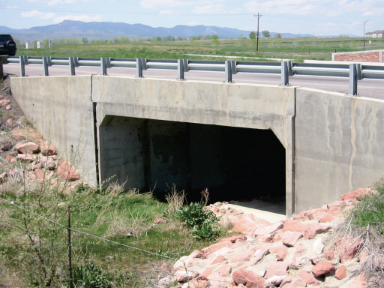
Figure 7‑2 Concrete box culvert (from FHWA, 2012)
Culvert flow can be controlled either by the inlet or the outlet. Inlet control occurs when the conveyance capacity of the culvert's barrel is higher than what the inlet will accept. Otherwise outlet control occurs, with the possibility that flow may be limited by backwater effects. Culverts are usually analyzed under a steady design flow condition to determine if the resulting inlet water depth will be acceptable. However for SWMM's unsteady dynamic wave analysis they are analyzed to find the flow corresponding to known inlet and outlet depths. (Culvert analysis is not made under kinematic wave analysis.)
Any SWMM conduit link can be designated as a culvert by assigning it one of the code numbers associated with a particular shape, material, and inlet configuration listed in Table H-1 in Appendix H. The choice made from the table should be consistent with the conduit's designated shape (circular, rectangular, ellipsoid, or arch). At any given time step of a simulation the flow through the culvert is first determined using SWMM's usual dynamic wave procedure. This flow represents the outlet control condition. Then an inlet controlled flow is computed to see if it becomes the limiting flow rate.
Under inlet control, a rating curve establishes the relationship between culvert flow rate and inlet head. The shape of the curve varies depending on the culvert's shape, material, and geometry of its inlet opening. Figure 7-3 shows a typical inlet control rating curve in normalized form, where inlet headwater depth (*Y1*) is normalized by the full barrel depth (*Yfull*) and flow rate (Q) is normalized by \(A_{full}\sqrt{Y_{full}}\) where *Afull* is the full cross-section area of the barrel. When the inlet is submerged it performs as an orifice while when unsubmerged it performs as a weir.
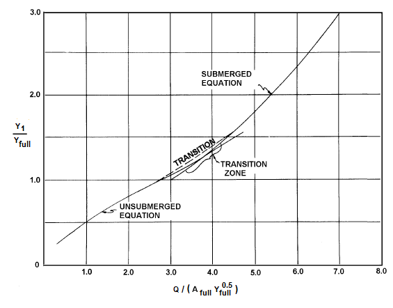
Figure 7‑3 Example of a culvert rating curve (from FHWA, 2012)
Based on extensive experimental testing done by the National Bureau of Standards, FHWA has developed inlet rating curves for a number of different types of culverts and their inlet configurations. The curves have been fitted to analytical functions that describe both their submerged and unsubmerged portions. Table H-1 in Appendix H lists the different types of culverts for which parameterized rating curves have been developed. Table H-2 lists the parameter values used for both the unsubmerged and submerged portions of each curve.
The FHWA procedures identify two types of unsubmerged curves used to compute inlet control for a culvert. The form 1 equation is:
\[\frac{H_{1} - Z_{1}}{Y_{full}} = \frac{E_{C}}{Y_{full}} + K_{I}\left\lbrack \frac{Q_{IC}}{A_{full}\sqrt{Y_{full}}} \right\rbrack^{M_{I}} + ScfS_{O}\]
(7-39)
while the form 2 equation is:
\[\frac{H_{1} - Z_{1}}{Y_{full}} = K_{I}\left\lbrack \frac{Q_{IC}}{A_{full}\sqrt{Y_{full}}} \right\rbrack^{M_{I}}\]
(7-40)
The following definitions apply to these equations:
H1 = hydraulic head at the inlet node of the culvert link (ft)
Z1 = elevation of the culvert invert at its inlet end (ft)
QIC = inlet controlled flow rate through the culvert (cfs)
EC = specific head at critical depth for flow QIC (ft)
Yfull = full depth of the culvert barrel (ft)
Afull = full area of the culvert barrel cross section (ft2)
SO = culvert barrel slope (ft/ft)
Scf = slope correction factor (0.7 for mitered inlets and -0.5 for all others)
KI, = constants from Table H-2 for corresponding culvert type in MI Table H-1.
Table H-2 also specifies which equation is used for each type of culvert. It should be noted that KI has a factor of \(g^{\frac{- M_{I}}{2}}\) embedded in it so that equations 7-39 and 7-40 are dimensionally consistent.
The form 2 equation can be solved directly to determine QIC for a given inlet head H1:
\[Q_{IC} = A_{full}\sqrt{Y_{full}}\left( \frac{H_{1} - Z_{1}}{K_{I}Y_{full}} \right)^{\frac{1}{M_{I}}}\]
(7-41)
For the form 1 equation, the specific head at critical depth is defined as:
\[E_{C} = Y_{C} + \frac{U_{C}^{2}}{2g}\]
(7-42)
where YC is the critical depth for flow QIC and UC is the velocity at this depth. From the definition of critical depth given by Equation 5-28 in Section 5.5.1:
\[U_{C}^{2} = g\frac{A\left( Y_{C} \right)}{W\left( Y_{C} \right)}\]
(7-43)
and from Equation 5-29:
\[Q_{IC} = A\left( Y_{C} \right)\sqrt{g\frac{A\left( Y_{C} \right)}{W\left( Y_{C} \right)}}\]
(7-44)
The area A and top width W values in these equations are evaluated at flow depth YC using the methods described in Chapter 5 that depend on the culvert's shape and dimensions.
Substituting these relations into the form 1 equation 7-39 results in the following nonlinear equation in the single unknown YC :
\[\frac{Y_{C}}{Y_{full}} = \frac{H_{1} - Z_{1} - \frac{Y_{HC}}{2}}{Y_{full}} - K_{I}\left\lbrack \frac{A\left( Y_{C} \right)}{A_{full}}\sqrt{g\frac{Y_{HC}}{Y_{full}}} \right\rbrack^{M_{I}} - ScfS_{O}\]
(7-45)
where \(Y_{HC}\) is the critical hydraulic depth defined as \(\frac{A\left( Y_{C} \right)}{W\left( Y_{C} \right)}\). This equation is solved using Ridder's root finding method (see Appendix B) with an initial bracket on YC of 10 to 100 percent of H1 – Z1 and a stopping tolerance of 0.001 ft. After YC is found the corresponding inlet control flow rate QIC can be computed using Equation 7-44.
The FHWA equation for inlet control of a culvert whose inlet is submerged is:
\[\frac{H_{1} - Z_{1}}{Y_{full}} = c_{I}\left\lbrack \frac{Q_{IC}}{A_{full}\sqrt{Y_{full}}} \right\rbrack^{2} + y_{I} + ScfS_{O}\]
(7-46)
where cI and yI are constants from Table H-2 for a particular culvert type in Table H-1. The cI constant has a factor of \(\frac{1}{g}\) embedded in it so that equation 7-46 is dimensionally consistent. Solving this expression for QIC results in:
\[Q_{IC} = \left\lbrack \left( \frac{1}{c_{I}} \right)\left( \frac{H_{1} - Z_{1}}{Y_{full}} - y_{I} - ScfS_{O} \right) \right\rbrack^{\frac{1}{2}}A_{full}\sqrt{Y_{full}}\]
(7-47)
The FHWA procedure states that the submerged inlet control equation should be used for values of \(\frac{Q_{IC}}{\left( A_{full}\sqrt{Y_{full}} \right)}\) above 4.0. Converting this into a condition on *H1* results in:
\[H_{1} > {H_{IS} = Z}_{1} + Y_{full}\left( 16c_{I} + y_{I} + ScfS_{O} \right)\]
(7-48)
When this condition is satisfied SWMM uses the submerged portion of the inlet control curve to compute the inlet control flow rate QIC.
FHWA states that the unsubmerged inlet control equation applies for \(\frac{Q_{IC}}{\left( A_{full}\sqrt{Y_{full}} \right)}\) values below 3.5. This is difficult to convert to an a priori limit on H1 because of the EC term in the form 1 unsubmerged equation. Therefore SWMM uses an arbitrary criterion of
\[H_{1} < {H_{IU} = Z}_{1} + 0.95Y_{full}\]
(7-49)
to determine if the unsubmerged inlet control equations should be used.
When H1 is between HIU and HIS linear interpolation is used to compute QIC as follows:
\[Q_{IC} = Q_{IC}\left( H_{IU} \right) + \left( Q_{IC}\left( H_{IS} \right) - Q_{IC}\left( H_{IU} \right) \right)\frac{\left( H_{1} - H_{IU} \right)}{\left( H_{IS} - H_{IU} \right)}\]
(7-50)
where \(Q_{IC}\left( H_{IU} \right)\) is the flow from the unsubmerged equation for a head of HIU and \(Q_{IC}\left( H_{IS} \right)\) is the flow from the submerged equation for a head of HIS.
SWMM's dynamic wave procedure needs to evaluate the derivative of a conduit's flow rate with respect to head (dQ/dH) for use when updating the head of a surcharged end node (see section 3.3.5). The derivatives for the various methods of computing an inlet control flow limit are as follows:
\[\frac{dQ_{IC}}{dH_{1}} = \left\{ \begin{matrix} \frac{Q_{IC}}{M_{I}H_{1}} & unsubmerged \\ \frac{0.5A_{full}^{2}}{c_{I}Q_{IC}} & submerged \\ \frac{Q_{IC}\left( H_{1S} \right) - Q_{IC}\left( H_{1U} \right)}{H_{1S} - H_{1U}} & transition \end{matrix} \right.\ \]
(7-51)
The following steps summarize how a culvert conduit is checked for inlet control each time that a new flow is computed for it under dynamic wave analysis:
A culvert will become overtopped when the headwater rises to the elevation of the roadway (see Figure 7-4). SWMM represents the flow across the road with a special type of weir link designated as a roadway weir. It is similar to a standard SWMM transverse rectangular weir but has its own specific methods for computing a weir coefficient and submergence factor based on road characteristics. Figure 7-5 shows how a roadway weir would be configured with a culvert in a SWMM node-link layout.
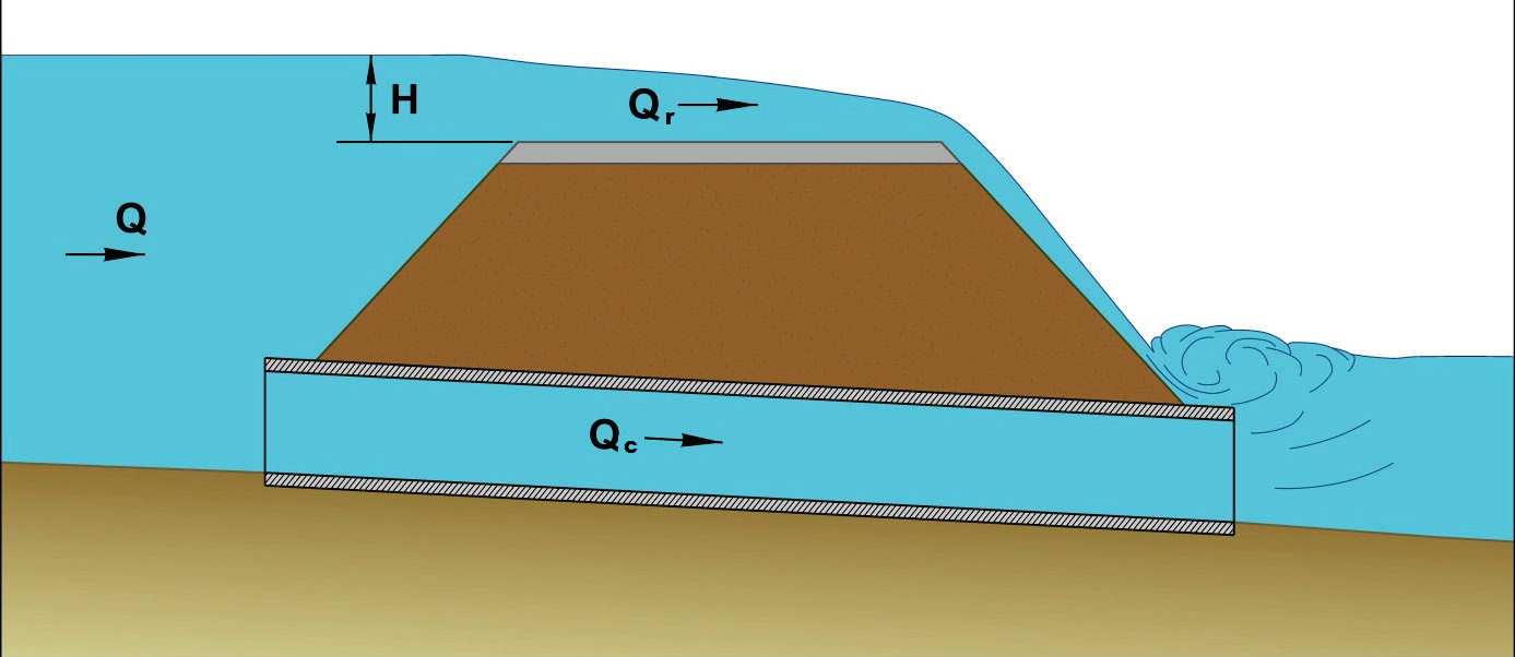
Figure 7‑4 Roadway overtopping (from FHWA, 2012)
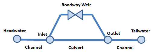
Figure 7‑5 SWMM node-link representation of a culvert with a roadway weir
The standard transverse rectangular weir equation can be used to compute the flow across a roadway weir as follows: (FHWA, 2012):
\[Q = {f_{S}C}_{W}LH^{3/2}\]
(7-52)
where Q is the overtopping flow rate (cfs), H is the height of the upstream water surface above the roadway crest (ft), L is the length of the roadway crest (ft), CW is free flow weir discharge coefficient (ft1/2/sec) and fS is a submergence adjustment factor.
Values for the flow coefficients CW and fS have been published by the FHWA as functions of the headwater depth (H), tailwater depth (ht), the width of the roadway (Lr), and road surface material. The functions are shown in graphical form in Figure 7-6.
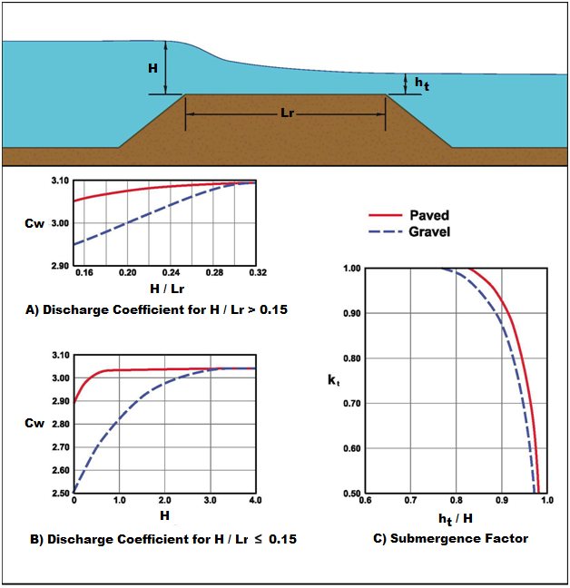
Figure 7‑6 Discharge coefficients for roadway weirs (from FHWA, 2012)
To summarize, SWMM includes an additional type of weir, a roadway weir, used to model flow over the top of a road that sits above a culvert or possibly an embankment. Its properties include the following:
Unlike the other weirs discussed in Chapter 6, a roadway weir has neither a control setting nor a flap gate. Its flow versus head relation is given by equation 7-52, where the head H is the difference between the head at its inlet node and its crest elevation, the tailwater head ht is the difference between its outlet node head and its crest elevation, and its flow coefficients are determined from the curves in Figure 7-6.
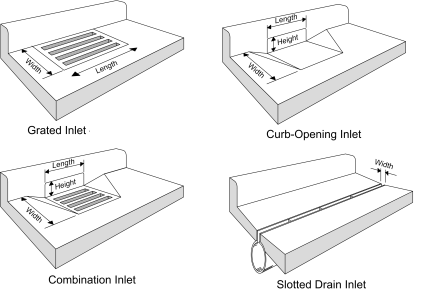
Storm drain inlets are structures that convey runoff from roadway pavements into below ground storm sewers (see Figure 7-7). Inlet type, sizing and spacing are normally chosen to meet limits on the spread and depth of water across a roadway as set by local drainage agencies to maintain public safety. The U.S. Department of Transportation Federal Highway Administration's Urban Drainage Design Manual (HEC-22) (FHWA, 2009) contains experimentally derived equations for computing the amount of flow captured by different types of inlets. These equations are widely used throughout North America and have been incorporated into SWMM's flow routing routines.
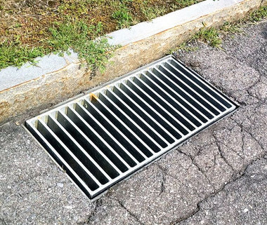 " @image{inline} html hydraulics/media/media/image60.png "CurbOpening.png"
Figure 7-7 Examples of storm drain inlets.
Figure 7-8 depicts the different types of street inlet structures whose hydraulic performance is computed using the HEC-22 procedures. In addition to these standard inlet types, a custom inlet can also be deployed. Its performance is defined by a user-supplied rating curve of captured flow as a function of flow depth, a diversion curve of captured flow as a function of flow upstream of the inlet, or both curves (see Figure 7-9). These curves are defined by a tabular listing of their data points.
Figure 7-8 Standard types of curb and gutter inlets
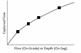
Figure 7-9 Performance curve for a custom inlet
To add storm drain inlet modeling into SWMM a site is represented as a dual drainage system consisting of both street conduits along the ground surface and sewer conduits below it as shown in Figure 7-10. An inlet structure will divert some portion of the street flow it sees into a designated node of the sewer system with the rest being bypassed to downstream streets. When an inlet's sewer node reaches its full depth any excess flow that would cause it to flood is sent back through the inlet and onto the street.
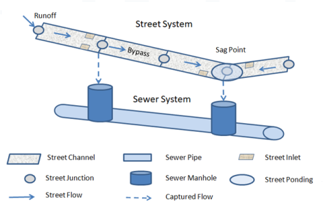
Figure 7-10 Representation of a dual drainage system
The HEC-22 procedures assume that the curb and gutter inlets shown in Figure 7-8 are placed in conduits that have a Street cross-section shape as described in Section 5.4. Even if a street conduit does not contain inlets, it should still be assigned a Street cross-section if the spread and depth of surface water across it needs to be reported. The Street cross-sections can be either single sided (have a single section that slopes downward from the street crown) or dual sided (have mirror image sloping sections on either side of the street crown) as required.
Streets can be assigned any number of a specific inlet design (grate, curb opening, combination, or slotted drain). If the cross-section is dual sided then each side receives the replicate number of inlets. If a street needs to use a mix of inlet designs then it needs to be divided into separate street conduits where each utilizes just a single type of design.
As shown in Figure 7-10, inlets can be located either on a continuous sloping section of roadway (on-grade) or at a low point where flow tends to pool (on-sag). The HEC-22 procedures make flow capture for on-grade inlets a function of the approach flow rate they see while flow capture for on-sag inlets depends on the depth of water that pools above them.
Because there is no physical link in the model, such as a shared manhole, weir or orifice, that connects the street and sewer system to one another, there is no need to have the rim elevation of a sewer manhole match the invert elevation of the street node that sends inlet flow into it.
To account for the flow capture and diversion provided by inlets, at each flow routing time step SWMM adjusts the lateral inflows seen at the downstream nodes of street conduits with inlets and at the sewer nodes designated to receive inlet flow. These lateral flows contribute to the node flow continuity equation 3-5 for dynamic wave routing and to the link flow continuity equation 4-8 for kinematic wave routing. The steps involved can be summarized as follows:
In Step 1, because each side of a two-sided street has the same cross-section geometry and number of inlets, flow capture is computed for only one side using half the total street flow as the approach flow seen by its inlets. The one-sided flow capture is then doubled to determine the full flow capture for the entire street.
The flow capture efficiency of an inlet placed on-grade is affected by:
Grate Inlets
For a standard street grate located on-grade the HEC-22 equation for flow capture is:
\[Q_{c} = Q\left\{ R_{f}E_{0} + R_{s}(1 - E_{0}) \right\}\]
(7-53)
where:
Qc = captured flow (cfs)
Q = approach flow (cfs)
E0 = ratio of flow over the grate's width to total flow
Rf = frontal capture efficiency
Rs = side capture efficiency
The frontal capture efficiency Rf is:
\[R_{f} = 1 - 0.09\ max(0,\ V - V_{o})\]
(7-54)
while the side capture efficiency Rs is:
\[R_{s} = 1/\left\{ 1 + 0.15V^{1.8}/(S_{x}L^{2.3}) \right\}\]
(7-55)
with:
V = velocity of flow over the grate (ft/sec)
V0 = velocity at which water begins to splash over the inlet (ft/sec)
Sx = street cross slope (ft/ft)
L = grate length (ft)
FHWA (2009) contains curves showing how the splash-over velocity V0 increases with increasing grate length L for the common grate designs listed in Table 7-5. Table 7-6 contains polynomial expressions that were fit to these curves by UDFCD (2010) that are used by SWMM. For grates that do not conform to one of the listed designs the splash-over velocity must be supplied by the user.
**Table 7-5 Description of grate inlet types1**
| Grate Type | Layout | Description |
|---|---|---|
| P-50 |
| Parallel bar grate with 1-7/8" bar spacing on center |
| P-50x100 | *[Figure image not available in this format]* | Parallel bar grate with 1-7/8" bar spacing on center and 3/8" diameter lateral rods spaced at 4" on center |
| P-30 | [Figure image not available in this format] | Parallel bar grate with 1-1/8" bar spacing on center |
| Curved Vane |  | Curved vane grate with 3-1/4" longitudinal bar and 4-1/4" transverse bar spacing on center |
| 45° Tilt Bar |  | 45° tilt-bar grate with 3-1/4" longitudinal bar and 4" transverse bar spacing on center |
| 30° Tilt Bar |  | 30° tilt-bar grate with 3-1/4" longitudinal bar and 4" transverse bar spacing on center |
| Reticuline |  | Honeycomb pattern of lateral bars and longitudinal bearing bars |
1See FHWA (2009) for more detailed descriptions and pictures.
**Table 7-6 Splash-over velocity for different types of grate inlets1**
| Grate Type | **Splash over velocity *V0* (ft/s) as a function of grate length L (ft)** |
|---|---|
| P-50 | \(V_{0} = 2.22 + 4.03L - 0.65L^{2} + 0.06L^{3}\) |
| P-50x100 | \(V_{0} = 0.74 + 2.44L - 0.27L^{2} + 0.02L^{3}\) |
| P-30 | \(V_{0} = 1.76 + 3.12L - 0.45L^{2} + 0.03L^{3}\) |
| Curved Vane | \(V_{0} = 0.30 + 4.85L - 1.31L^{2} + 0.15L^{3}\) |
| 45° Tilt Bar | \(V_{0} = 0.99 + 2.64L - 0.36L^{2} + 0.03L^{3}\) |
| 30° Tilt Bar | \(V_{0} = 0.51 + 2.34L - 0.20L^{2} + 0.01L^{3}\) |
| Reticuline | \(V_{0} = 0.28 + 2.28L - 0.18L^{2} + 0.01L^{3}\) |
1 Source: Denver UDFCD (2010).
Curb Opening Inlets
For a curb opening inlet located on-grade, the HEC-22 equation for flow capture is:
\[Q_{c} = Q\left\{ 1 - {(1 - min(1,\ L/L_{T})\ )}^{1.8} \right\}\]
(7-56)
L is now the length of the curb opening and LT is the length at which complete flow capture occurs. The latter quantity is computed as:
\[L_{T} = 0.6Q^{0.42}S_{L}^{0.3}{(nS_{e})}^{- 0.6}\]
(7-57)
where:
SL = longitudinal street slope (ft/ft)
n = Manning's roughness coefficient for the street surface
Se =
\[S_{x} + (\frac{a}{W)E_{0}}\]
a = curb depression (ft)
W = depressed gutter width (ft)
E0 = ratio of flow over depressed gutter width to total flow
If L > LT then complete capture is obtained.
Computing E0
The on-grade flow capture formulas for grate and curb opening inlets need to know Eo, the fraction of total street flow Q within a distance W from the curb or as depicted in Figure 7-11, the ratio of QW to Q. For grates this distance is the width of the grate. For curb openings it is the width of the depressed gutter (if present).
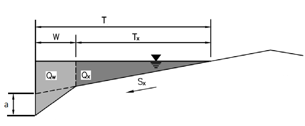
Figure 7-11 Street cross-section divided into gutter and roadway flow
HEC-22 bases its determination of *E0* on Izzard's form of the Manning equation that relates flow spread T to flow rate Q for a triangular cross-section. It is derived from the standard Manning equation by integrating the hydraulic radius across successive increments of street width. The result for US standard units is:
\[Q = (\frac{0.56}{n)S_{x}^{1.67}S_{L}^{0.5}T^{2.67}}\]
(7-58)
(Note: the standard Manning equation has the same form except with the constant being 0.47.)
Solving for T as a function of Q gives:
\[T = \left\lbrack \frac{Qn}{0.56S_{x}^{1.67}S_{L}^{0.5}} \right\rbrack^{0.375}\]
(7-59)
If the street has a uniform cross slope ( \(a = 0\) in Figure 7-12) then Equation 7-59 can be used to derive the following expression for*E0*:
\[E_{0} = 1 - {(1 - \frac{W}{T})}^{2.67}\]
(7-60)
where T is evaluated at a given flow rate Q.
For a compound street cross-section with depressed curb ( \(a > 0\) in Figure 7-12), HEC-22 provides the following equation for *E0*:
\[E_{0} = \frac{1}{1 + \frac{\frac{S_{W}}{S_{X}}}{\left\lbrack 1 + \frac{\frac{S_{W}}{S_{X}}}{\left( \frac{T}{W} - 1 \right)} \right\rbrack^{2.67} - 1}}\]
(7-61)
where \(S_{W} = S_{X} + \frac{a}{W}\). It is not possible to solve directly for E0 since Equation 7-59 for T(Q) applies only to a triangular section of uniform slope.
To solve equation 7-61 let QX and TX denote the flow and spread, respectively, across the non-depressed triangular portion of the street's cross section. Then the following relations apply:
\[Q_{X} = Q(1 - E_{0})\]
(7-62)
\[T_{X} = T - W\]
(7-63)
\[\frac{T}{W} - 1 = \frac{T_{X}}{W}\]
(7-64)
These can be used in the following iterative procedure to find E0 for a particular flow rate Q:
In cases where the width of the grate is smaller than the width W of the depressed gutter section, E0 is adjusted by the ratio of the flow area over the grate's width to the flow area over the depressed gutter width.
Combination Inlets
A combination inlet consists of both a grate and curb opening placed together at the same location. Its on-grade flow capture equals that of the grate plus any flow captured by the portion of the curb opening that extends upstream of the grate's length. The latter flow capture is computed first and is subtracted from the approach flow used to determine the grate's flow capture.
Slotted Inlets
The flow capture capability of a slotted inlet located on-grade is the same as that of a curb opening inlet of equal length.
Custom Inlets
If an on-grade custom inlet is supplied with a flow diversion curve (captured flow v. approach flow) then that curve will be used to determine its flow capture. If it only has a flow rating curve (captured flow v. water depth) then that curve will be used in conjunction with the water surface depth at the downstream end of the conduit containing the inlet.
HEC-22 has flow capture efficiency for an inlet in a sag location depend on the size of the inlet's opening and the depth of water that collects next to it at the street curb. At low flow depths the inlet acts as a weir with
\[Q_{c} = C_{W}L_{W}d^{1.5}\]
(7-66)
while at higher depths it acts as an orifice with
\[Q_{c} = C_{O}A_{O}\sqrt{2gd}\]
(7-67)
In these equations:
CW = weir coefficient (ft0.5/sec)
CO = orifice coefficient
g = acceleration of gravity (ft/sec2)
LW = effective length of inlet (ft)
AO = open area of inlet (ft2)
d = effective depth of water seen by the inlet (ft).
Grate Inlets
For grate inlets the following values are used in Equations 7-66 and 7-67:
CW = 3.0
CO = 0.67
Lw = L + 2W
AO =
\[LWf_{O}\]
d =
\[d_{i} - (\frac{W}{2)S_{W}}\]
where L is the grate's length, W its width, fO the ratio of open area to full area, and di is the depth of water at the downstream node of the conduit containing the inlet. Opening ratios for several types of grate designs are listed in Table 7-5.
HEC-22 does not provide clear guidance on what depth causes a switch from weir flow to orifice flow for grates. Therefore it is assumed the switch occurs at a depth d where Equation 7-66 equals Equation 7-67. This results in weir flow for depths below \(1.79\frac{A_{O}}{L_{W}}\) and orifice flow for depths above it.
Curb Opening Inlets
For streets with uniform cross slope or for openings greater than 12 feet in length, the values used in Equation 7-66 for weir flow are CW = 3.0 and LW = opening length. Otherwise, CW = 2.3 and \(L_{W} = L + 1.8W\) where L = opening length and W = width of the depressed gutter. The values used in Equation 7-67 for orifice flow are \(C_{O} = 0.67\) and \(A_{O} = hL\) where h is the height of the opening. The effective depth d seen by the curb opening inlet under orifice flow depends on the orientation of the opening's throat relative to the street surface as shown in Table 7-7.
Table 7-7 Effective depth for curb opening inlets under orifice flow
| Throat Angle | Image | Effective Depth |
|---|---|---|
| Horizontal |
| \(d = d_{i} - \frac{h}{2}\) |
| Inclined |
| \(d = d_{i} - 0.7071(\frac{h}{2})\) |
| Vertical |
| \(d = d_{i}\) |
HEC-22 states that weir flow for on-sag curb openings occurs at effective depths below h while orifice flow occurs at depths greater than 1.4h. For depths in between these SWMM uses the following interpolation formula:
\[Q_{c} = (1 - r)Q_{weir} + rQ_{orif}\]
(7-68)
where Qweir is weir flow capture at depth h, Qorif is orifice flow capture at depth 1.4h and \(r = \frac{(d - h)}{(0.4h)}\).
Slotted Inlets
For slotted inlets the variables in the weir and orifice equations 7-66 and 7-67 are as follows:
CW = 2.48
CO = 0.8
Lw = L
AO =
\[LW\]
di =
\[d\]
where L = inlet length and W = inlet width. Weir flow holds for \(d \leq 0.2\) feet while orifice flow occurs for \(d \geq 0.4\) feet. In between these values flow capture is computed using Equation 7-68 with Qweir as weir flow capture at depth 0.2, Qorif as orifice flow capture at depth 0.4 and \(r = \frac{(d - 0.2)}{0.2}\).
Custom Inlets
If an on-sag custom inlet is supplied with a flow rating curve (captured flow v. water depth), then that curve is used to determine its flow capture. The depth supplied to the curve's lookup table is the depth of the downstream node of the conduit containing the inlet. If the inlet was only assigned a diversion curve (captured flow v. approach flow) then that curve is used thus essentially treating the inlet as if it were on-grade.
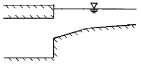
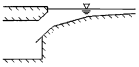
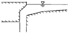
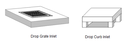
Drop inlets, pictured in Figure 7-12, are used to drain water from roadside ditches, swales and flat bottom channels. SWMM allows these structures to be placed in open channels that have either a rectangular or trapezoidal cross-section. Model set-up for utilizing these inlets is the same as described in section 7.6.2 and the same computational scheme applies. The methods used to compute their flow capture efficiencies are described in the following paragraphs.
Figure 7-12 Types of channel drop inlets
Drop Grate Inlets
The flow capture equation for a drop grate inlet located on-grade is the same as for a street grate (see equation 7-53) except that the ratio *E0* of flow over the grate to total cross-section flow Q is given by:
\[E_{0} = \frac{1.486\sqrt{S_{L}}{(yW)}^{1.67}}{nQ{(W + 2y)}^{0.67}}\]
(7-69)
where
W = side length of grate parallel to flow direction (ft)
y = flow depth in the channel (ft)
n = channel Manning's roughness coefficient
SL = channel longitudinal slope (ft/ft)
A cross slope SX of 1% is assumed unless the grate extends across the entire bottom width of a trapezoidal channel. In that case SX is taken as the slope of the channel's side wall.
Drop grates located on-sag use the same weir and orifice equations (7-66 and 7-67) as do street grates with the only difference being that for weir flow the effective length of the inlet's sides (LW in equation 7-66) is the sum of the lengths of all four sides.
Drop Curb Inlets
Flow capture for drop curb inlets is computed the same as for curb opening inlets located on sag. The only difference is that the effective length of the opening is the total length of all four sides and the open area is the height of the opening times the total length of all four sides.
 1.13.2