 |
OpenSWMM Engine
6.0.0-alpha.4
Data-oriented, plugin-extensible SWMM Engine (6.0.0-alpha.4)
|
|
OpenSWMM Engine
6.0.0-alpha.4
Data-oriented, plugin-extensible SWMM Engine (6.0.0-alpha.4)
|
As mentioned in Chapter 1, SWMM models the conveyance portion of a drainage system as a network of links connected together at nodes. External flows from various sources enter the network at specific nodes, are transported along links, are combined together and split apart at internal nodes while filling and emptying the volume of storage nodes, and exit the system at terminal nodes. Figure 2-1 shows how a physical system of sewer lines and their appurtenances are abstracted into a network of nodes and links of different types (pipe and pump links; junction, storage and outfall nodes for this particular example).
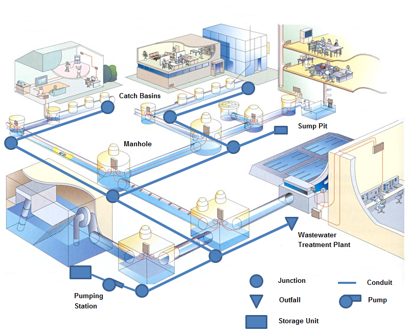
Figure 2-1 Node-link representation of a sewer system (Background from http://www.sewerhistory.org/photosgraphics/japan/)
Table 1-2 has already summarized the different types of node and link objects that can appear in a SWMM conveyance network model. The remainder of this chapter provides more details on the properties of network objects, briefly describes and compares the capabilities of the two principal methods used for analyzing the unsteady hydraulic behavior of a network, and discusses the boundary and initial conditions needed to compute network hydraulics.
The two principal components of a SWMM conveyance system network are nodes and links. Nodes represent the end points of conveyance links that form the connection between two or more links. They are also the points where external inflows (runoff, dry weather flows, etc.) can enter the network or where internal flows leave the network. Links are conveyance elements that transport flow between nodes. The following paragraphs describe the different types of nodes and links that SWMM can model.
Junction nodes are points in the drainage system where conveyance links join together. Physically they can represent the confluence of natural surface channels, manholes in a sewer system, or pipe connection fittings. Excess water at a junction can become partially pressurized when connecting conduits are surcharged and can either be lost from the system or be allowed to pond atop the junction and subsequently drain back into the junction.
The principal input parameters for a junction node are:
Outfall nodes are terminal nodes of the drainage system used to define final downstream boundary locations. The boundary conditions at an outfall can be described by any one of the following stage relationships:
The principal input parameters for an outfall node are:
Flow divider nodes divert inflows to a specific link in a prescribed manner. A flow divider can have no more than two conduit links on its discharge side. There are four types of flow dividers, defined by the manner in which inflows are diverted:
The principal input parameters for a flow divider node are:
Storage unit nodes are the only type of node that can provide storage volume and possess surface area. Physically they could represent storage facilities as small as a catch basin or as large as a lake. The volumetric properties of a storage unit are described by a function or table of surface area versus height. In addition to receiving inflows and discharging outflows to other nodes in the drainage network, storage nodes can also lose water from surface evaporation and from seepage into native soil. Unlike other nodes, storage nodes are not allowed to pressurize (i.e., they always maintain a free surface).
The principal input parameters for a storage unit are:
Conduit links are pipes or channels that move water from one node to another in the conveyance network. Their cross-sectional shapes can be selected from a variety of standard open and closed geometries. Custom closed shapes for pipes and irregular cross-section profiles for open channels can also be specified. Conduit geometry is discussed in more detail in Chapter 5.
The required input parameters for a conduit link are:
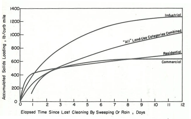
SWMM allows conduits to be offset some distance above the invert of their connecting end nodes as shown in the figure on the right. The offset can be specified as either a distance above the invert (i.e., the distance between points 1 and 2 in the figure) or as the elevation of the conduit's invert (i.e., the elevation of point 1). Internally the offset is maintained as an elevation.
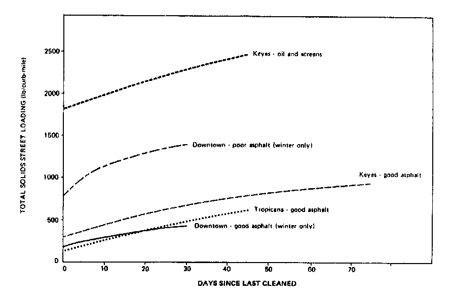
SWMM also makes use of a conduit's slope in its hydraulic calculations. Slope is not provided directly as an input variable but is instead computed from the elevation of a conduit's end node inverts and its offsets. Let L be the length of the conduit, ∆y be the difference in elevation and ∆x the horizontal distance between the invert at each end of the conduit. Then from the diagram on the right:
∆x = √(L2 - ∆y2) (2-1)
and the conduit slope S0 is:
S0 = ∆y/*∆x* (2-2)
SWMM does not allow a slope of 0. Therefore it imposes a minimum value of 0.001 ft on ∆y. It also allows the user to set a non-zero value for minimum slope which will override any smaller computed slope.
SWMM uses the Manning equation to relate conduit flow rate to flow depth and conduit bed or friction slope. It therefore requires the user to supply a Manning's "*n*" coefficient that represents the roughness characteristics of the conduit's surface. Values of the coefficient for a wide range of channel types and pipe materials can be found in Appendix G.
Conduits can also include the following optional parameters:
The latter three properties are employed by the advanced modeling features covered in Chapter 7 of this manual.
Pump links are used to lift water from an inlet node to an outlet node at higher elevation. The principal input parameters for a pump include:
A pump curve describes the relation between a pump's flow rate and the head at its inlet and outlet nodes. The inlet node's startup and shutoff water depths are monitored continuously during the course of a simulation to allow for automated control of the pump's on/off status.
Pumps are directional devices that are not allowed to have reverse flow through them. Their hydraulic performance is described in more detail in Chapter 6.
Flow regulator links model structures or devices used to control and divert flows within a conveyance system. They are typically used to control releases from storage facilities, prevent unacceptable surcharging, and divert flow to treatment facilities and interceptors.
SWMM can model the following types of flow regulators: orifices, weirs, and outlets. The hydraulic behavior of orifices and weirs is modeled using standard rating curves (the nonlinear relation between hydraulic head applied to the regulator and the flow rate through it). Outlets utilize a user-supplied rating curve.
The principal input parameters for a flow regulator link include:
The hydraulic performance of regulator links is described in more detail in Chapter 6.
Each pump and flow regulator has a setting property that can adjust:
The setting can be changed during a simulation by using control rules. These specify conditions, such as water elevation at certain nodes, flow in certain links, and simulation time, that trigger a specified change in a link's setting. SWMM's hydraulic analysis methods take into account the current setting for each pump and flow regulator in the conveyance network. More details on the formats used for control rules can be found in the SWMM 5 Users Manual (US EPA, 2010).
SWMM's hydraulics solves the equations of one-dimensional, gradually varied, unsteady flow throughout a node-link network to determine the water level at each node and the flow rate and flow depth within each link at each time step of an extended simulation period. Flow routing of inflow hydrographs along channels and sewers entails wave dispersion, wave attenuation or amplification, and wave retardation or acceleration. These wave characteristics constitute the hydraulics of flow routing or propagation and are greatly affected by the geometric characteristics of the conduits, the characteristics of sources and/or sinks, and by initial and boundary conditions.
The hydraulics of unsteady non-uniform flow is represented in SWMM by a pair of partial differential equations of conservation of mass and momentum known as the St. Venant equations. Simultaneous solution of these equations for each conduit, coupled with a conservation of volume at each node, provides information on the spatial and temporal variation of water levels and discharge rates throughout the network. SWMM offers the user two principal alternative methods for solving these equations - dynamic wave or kinematic wave analysis
Dynamic wave analysis solves the complete form of the St. Venant flow equations and therefore produces the most theoretically accurate results. It can account for channel storage, backwater effects, entrance/exit losses, culvert flow, flow reversal, and pressurized flow. Because it couples together the solution for both water levels at nodes and flow in conduits it can be applied to any general network layout, even those containing multiple downstream diversions and loops. It is the method of choice for systems subjected to significant backwater due to downstream flow restrictions and with flow regulation via weirs and orifices. This generality comes at a price of having to use small time steps to maintain numerical stability.
Kinematic wave analysis solves the continuity equation along with a simplified form of the momentum equation in each conduit. It cannot account for backwater effects, entrance/exit losses, flow reversal, or pressurized flow. It is most applicable to steeply sloped (e.g., > 0.1%) conduits with shallow flow with high velocity. It can usually maintain numerical stability with much larger large time steps than are required for dynamic wave analysis. If the aforementioned effects are not expected to be significant then this alternative can be an accurate and efficient hydraulic analysis method, especially for long-term simulations.
Because kinematic wave analysis ignores both inertial and pressure forces there are limits on its applicability:
SWMM also offers a steady flow analysis option which assumes that within each computational time step flow is uniform and steady. It simply translates inflow hydrographs at the upstream end of a conduit to its downstream end, with no delay or change in shape. The Manning equation is used to relate flow rate to flow area (or depth). It is subject to the same limitations as the kinematic wave method. Because it ignores the dynamics of free surface wave propagation it is only appropriate for rough preliminary analysis of long-term continuous simulations.
Table 2-1 compares the features and limitations of the dynamic wave and kinematic wave methods of hydraulic analysis. Dynamic wave solutions tend to attenuate and disperse an inflow hydrograph as it routed downstream through a series of conduits while kinematic wave solutions show no attenuation, no dispersion, and some distortion of the hydrograph shape. This behavior is depicted in Figure 2-2 from Miller (1984) which shows the results of routing an inflow hydrograph down a 100-foot wide rectangular channel of 1% slope with a Manning's n of 0.06.
| Feature | Dynamic Wave | Kinematic Wave |
|---|---|---|
| Network topology | branched and looped | branched only |
| Flow splits | yes | with flow divider nodes |
| Adverse slopes | yes | no |
| Invert offsets | yes | ignored |
| Pumping | yes | only from storage nodes |
| Weirs and orifices | yes | only from storage nodes |
| Ponded overflows | yes | yes |
| Lateral seepage | yes | yes |
| Evaporation | yes | yes |
| Minor losses | yes | no |
| Culvert analysis | yes | no |
| Hydrograph attenuation | yes | no |
| Backwater effects | yes | no |
| Surcharge / Pressurization | yes | no |
| Reverse flow | yes | no |
| Tidal effects | yes | no |
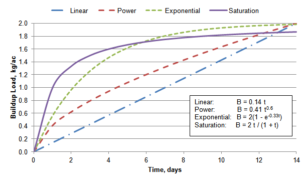
Figure 2-2 Comparison of dynamic wave and kinematic wave solutions (from Miller, 1984)
There are two types of boundary conditions that a user must supply to a SWMM conveyance network model:
Both types of conditions can vary with time. Outfall node heads are only required for dynamic wave analysis. The options available for specifying their values were described in Section 2.1.2. External inflows can originate from any of the following sources:
Time-dependent runoff, groundwater, and RDII inflows are normally provided by SWMM's hydrology module (see Volume I). It automatically links the computed flow from each of these sources at each time period to their designated receiving node. (Each SWMM subcatchment object that generates runoff is assigned a conveyance system node that receives this runoff. See Figure 1-2.)
User-defined external inflows can be attached to any node of the network. They are typically used to describe dry weather sewage flows in sanitary sewer systems, base flows in natural stream channels, or inflows in the absence of any hydrologic modeling. They are expressed in the following general format:
Flow rate at time t = (baseline value) × (baseline pattern factor) + (scale factor) × (time series value at time t)
The baseline value is some constant. The baseline pattern is a combination of repeating hourly, daily, and monthly multiplier factors applied to the baseline value. The time series value is a time varying value and the scale factor is a constant multiplier applied to each time series value. Time series values can be specified at unequal intervals of time with interpolation used to obtain values at intermediate times.
A set of initial conditions at time 0 for all node heads and link flows in the conveyance network must be specified before a hydraulic analysis can begin. The default is to set all these values to 0, with the user having the option to specify initial heads at selected nodes and initial flow rates in selected conduit links.
Any initial flow rate assigned to a conduit link is assumed to represent a uniform steady flow. Therefore its flow depth can be set to the normal depth determined by the Manning equation as described in Section 5.5.2. From this depth an initial cross-section flow area for the conduit can be found which is required for kinematic wave analysis.
For dynamic wave analysis, if a non-storage, non-outfall node has not had an initial head assigned to it then it's initial head is set equal to the average elevation of the initial flow depths in the conduits that deliver flow into it.
 1.13.2