This worked comparison accompanies Chapter 9: Two-Dimensional Overland Flow Analysis §9.7.1. It checks the implemented exchange equations against the 36 steady measurements of Rubinato et al. (2017) and demonstrates nine synthetic surcharge events. Experimental qualification remains incomplete. The synthetic forcing is not a replay of the measured transient events.

Report, data and runnable models

The downloads preserve the 21 October 2026 CPU comparison. The PDF retains its original review-draft label as the dated evidence record. Numerical results identify the pinned engine library in the JSON manifest; they are not assertions about every later engine build. The original checkout was dirty, so the recorded repository identifier alone is not a clean release.

Extract the examples into a working folder and open model.inp for the synthetic T9 demonstration. steady_s1.inp through steady_s4.inp are the first measured row of each steady scenario. All files are self-contained SI inputs with an inline mesh. Only MH is mapped to the surface; IN and OUT supply pipe boundary conditions and are explicitly not coupleable.

Laboratory configuration and comparison method

The no-lid physical model has a 0.24 m manhole linking a 75 mm pipe to an 8 m by 4 m flume, with slope 0.001 and Manning n = 0.009. The crest is 0.478 m above the pipe invert. Surface and pipe pressure measurements are 0.46 m and 0.35 m from the manhole centre respectively.

Scenario	Rows	Governing experimental regime
S1	15	Free-weir surface-to-sewer drainage
S2	5	Submerged-weir surface-to-sewer drainage
S3	8	Sewer discharge onto a wet surface
S4	8	Sewer discharge with no incoming surface flow

Both numerical reconstructions place MH at the flume centre and use a 1,600-triangle mesh with nominal 0.2 m spacing. This is not the authors' 11,186-cell mesh. A short, wide pipe to a fixed-stage outfall imposes the measured sewer pressure approximately. It represents an artificial pressure reservoir, rather than the complete laboratory sewer system.

Surface inflow is reconstructed as \(Q_1=Fr_s\sqrt{g h_s}\,h_s W\), assuming representative uniform flow across width \(W\). S4 has zero surface inflow. The Table 2 surcharge fraction defines \(Q_3=|Q_e/(p/100)|\) for S2-S4; S1 has no sewer inflow. The pipe Reynolds number must not be substituted for inlet flow. These reconstructed boundary conditions reuse the calibration observations; this is not an independent blind prediction.

The junction reconstruction uses the numerical node-area floor of about 1.167 m². The physical-shaft alternative books cylindrical storage below the rim and sets MIN_SURFAREA to the actual shaft area, 0.0452389 m². It changes storage and the area floor together, without retuning any exchange coefficient. Storage nodes retain their storage curves.

Physical-time smoothing follow-up — 22 October 2026

The opt-in THETA_REFERENCE_STEP keeps the numerical momentum relaxation rate tied to a fixed time interval. The new study holds THETA 0.8 and THETA_REFERENCE_STEP 1 fixed across 36 physical-shaft cases at routing steps 0.0125, 0.00625 and 0.003125 s (108 completed runs). It uses maximum 1D trials 80, head tolerance 0.00001 m, variable step 0 and lengthening step 0. Mesh, geometry, reconstructed forcing and physical coefficients are unchanged. The 1 s reference is a declared numerical timescale, not a fit to observations.

All 36/36 cases change by less than 1% between the two finest steps; the largest change is 0.516%. All pass the separate 2% successive-minute drift and ordinary 1D continuity checks. These are fixed-mesh temporal and numerical diagnostics. 0/36 fine-step results meet the illustrative experimental band, so experimental qualification remains incomplete. Stable rates expose substantial surcharge overprediction and submerged-regime errors that the original coarse-step comparison obscured.

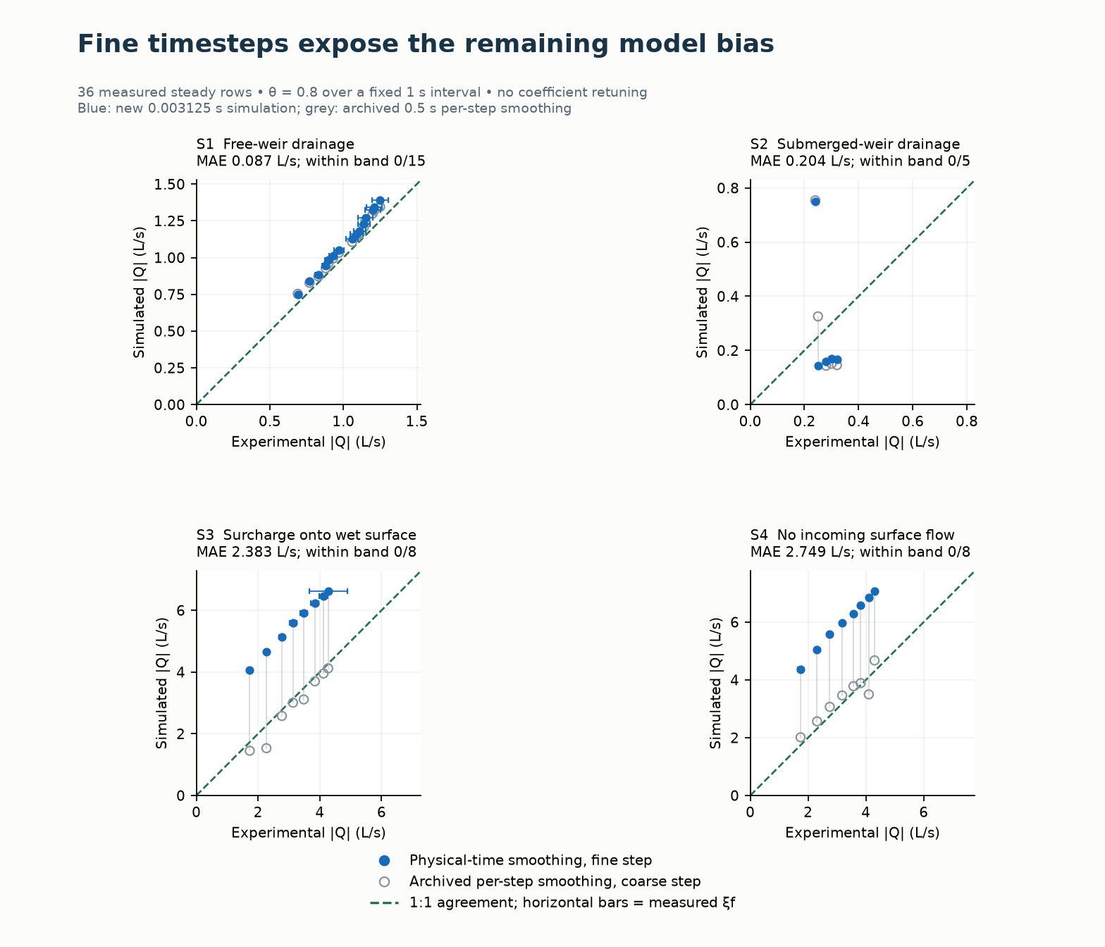
Physical-time smoothing compared with measured exchange

Blue filled circles show the new simulated rates at 0.003125 s; gray open circles show the archived physical-shaft results at 0.5 s with per-firing smoothing. The green dashed line is 1:1 agreement. Horizontal bars show measured variation. Both numerical schedules and their timesteps differ; this overlay does not isolate just one parameter.

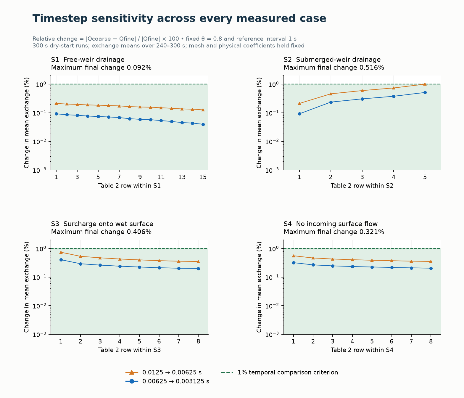
All-row timestep comparison with a fixed smoothing interval

Orange triangles show the first timestep halving, blue circles the final halving, and green shading the region below 1%. The ordinate is logarithmic. This check does not establish spatial convergence or independent validation.

Download the follow-up report, figures and plotted data, all 36 rows at three steps, or heads, separate volume ledgers and binary/source identifiers. The previous report, plots and synthetic transient viewer remain the dated 21 October record. Their outputs have not been replaced by new transient runs.

To reproduce the new mode, hold the reference interval fixed while refining the routing step. Zero or omission retains the historical per-firing blend. Positive values are persisted and checked in restart compatibility; surface plugins require GPU ABI 9. See Chapter 9: Two-Dimensional Overland Flow Analysis §9.5.1 for the retention equation. Further experimental work should resolve the boundary/head reconstruction and spatial delivery before coefficient fitting.

Absolute steady agreement — 21 October archive

The following ranges use all rows of each scenario. Bias is \(100(|Q_{model}|/Q_e-1)\). The bare paper equations use measured heads; the two reconstructions evolve the surface and node heads. The routed runs use WEIR_ORIFICE, STENCIL_WET_MEAN, RUBINATO2017, a 0.5 s routing step, and a 300 s dry-start simulation. Rates are measured over 240-300 s.

Scenario / rows	Paper-equation bias (%)	Junction bias (%)	Shaft bias (%)
S1 / 15	+8.3 to +17.7	+4.4 to +9.2	+4.4 to +9.2
S2 / 5	-23.3 to -17.3	-48.1 to +214.6	-54.4 to +214.3
S3 / 8	+58.5 to +144.6	+57.3 to +144.1	-32.5 to -3.6
S4 / 8	+84.1 to +208.3	+65.0 to +154.4	-14.7 to +15.7

Only 8/36 physical-shaft rates meet the illustrative band \(|Q_{model}-Q_e|\leq\xi_f+0.02Q_e\). None of the 36 bare zero-intercept paper-equation values meets that band. This band is a fit diagnostic, not a statistical confidence interval or an engine verification tolerance.

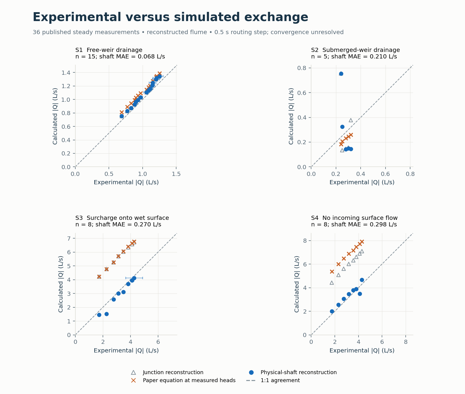
Experimental versus simulated steady exchange

Each panel pairs every measured Table 2 rate with the corresponding model rate. Horizontal bars show the published \(\xi_f\) variation at the physical-shaft points; the dashed line is 1:1 agreement. Each panel has equal x/y scales, but scales differ between regimes. MAE is the mean absolute physical-shaft residual in L/s. The paper-equation series uses measured heads; the full-engine series evolves the heads.

Steady exchange residuals

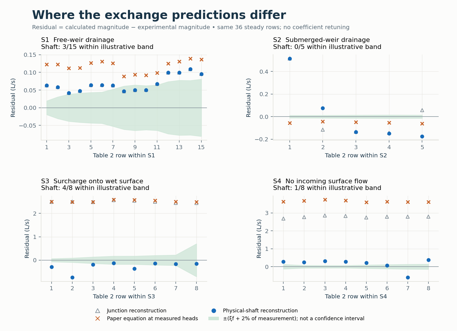
Residuals are calculated minus experimental discharge magnitudes. Green shading shows the illustrative \(\pm(\xi_f+0.02Q_e)\) band. Case numbers restart within each scenario. This is a comparison of calibration rows, not independent experimental validation. No coefficient was retuned.

The paper's Table 3 coefficients are slopes of fits with nonzero intercepts. Regressing the rounded Table 2 data recovers slopes of about 0.534, 0.061, 0.165 and 0.163 for S1-S4, with intercepts -0.105, +0.033, -2.461 and -3.797 L/s. Matching slopes and high R-squared therefore does not establish absolute discharge agreement. The implementation's inward orifice coefficient is borrowed by analogy; that regime was not calibrated by these experiments. See §9.7.1 for the exact preset mapping.

Numerical checks and routing-step sensitivity — 21 October archive

The physical-shaft alternative puts all 36 ordinary 1D continuity errors within 2%, but five cases fail a 2% successive-minute drift check. The original junction reconstruction has large continuity errors. The broader suite records 59 numerical passes and 56 numerical failures, with no execution errors; these counts include the original junction and legacy comparison cases. Observed-flow fit is reported separately.

One case per scenario was selected by its largest 0.5 s window drift. Reducing the routing step to 0.05 s stabilises the late windows but changes mean exchange substantially. Signed rates below are positive to the surface.

Selected case	Q at 0.5 s (L/s)	Q at 0.05 s (L/s)
S1_8_SHAFT	-1.106	-0.951
S2_2_SHAFT	-0.326	-0.137
S3_1_SHAFT	+1.449	+3.799
S4_7_SHAFT	+3.498	+6.649

These two-step sensitivities are not a time-convergence study. Apparent agreement at the coarser step must not be used to claim validation or to calibrate coefficients. The complete steady table remains a 0.5 s diagnostic.

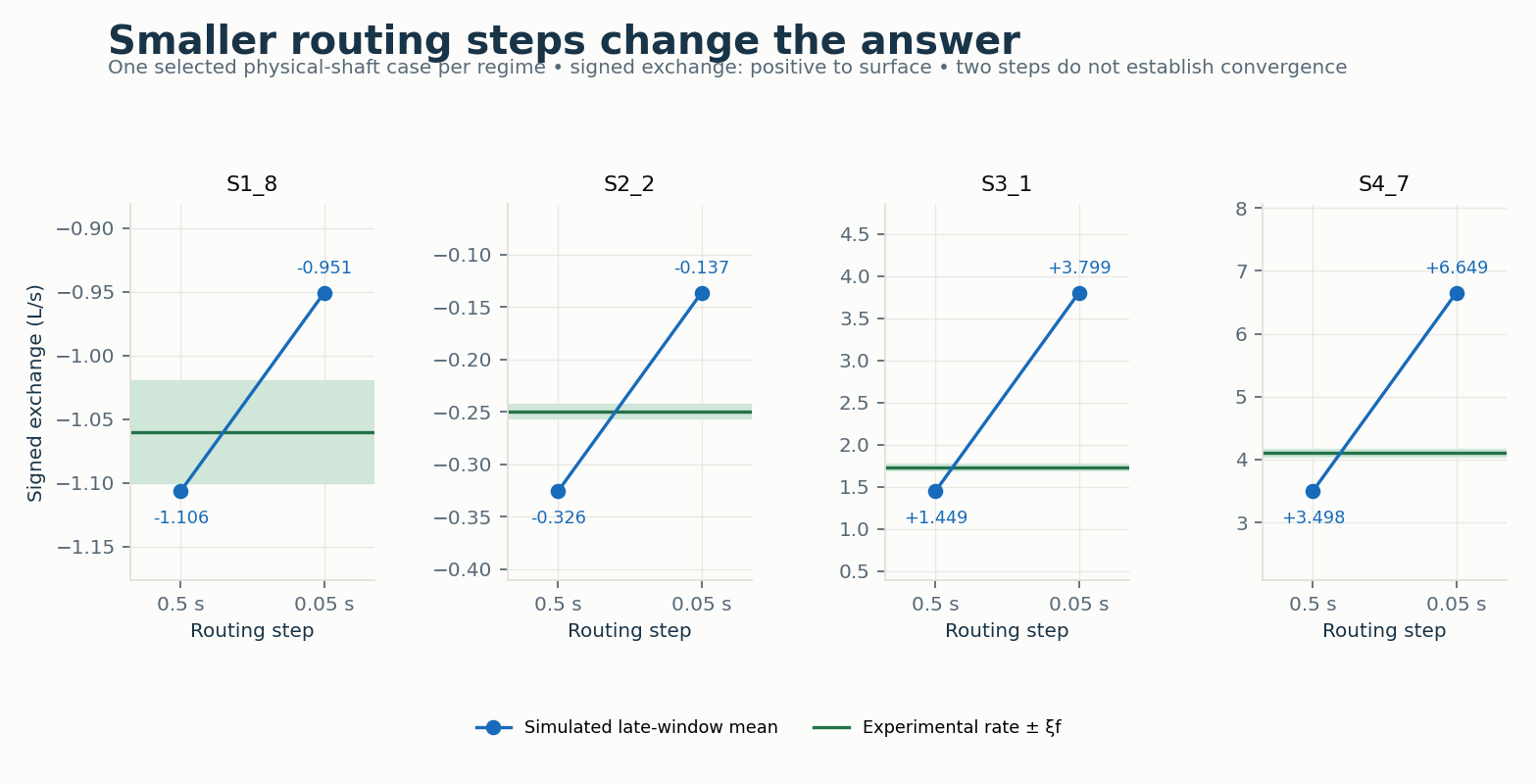
Experimental rates and routing-step sensitivity

Green lines and bands show each selected experimental rate and \(\xi_f\); blue points are the simulated late-window means. Signed rates are positive to the surface. Only these four cases were rerun at 0.05 s.

The fine-mesh anti-choking check has 9,600 cells and nominal 0.0125 m grid spacing near the manhole. Equalisation on/off yields about 3.4146 L/s in both runs, but the ordinary 1D continuity error is about 35.93%. Passing this anti-choking check does not establish spatial convergence. Exchange is delivered to one cell even when the opening covers several cells.

Synthetic transient demonstration

The nine synthetic events use Table 1's peak ratios and durations, constant surface inflow 8.15 L/s, a 30 s rise beginning at 60 s, a plateau, and a 30 s fall. Runs last 600 s. The downstream stage is explicitly assumed to be 0.45 m. Timeseries entries are HH:MM:SS; two fields would be interpreted as hours and minutes and had placed the pulse outside the run.

All 27 lower/expected/upper-preset runs complete and pass the numerical checks: nonnegative depths, both transfer directions, at least two reversals, and ordinary 1D continuity within 2%. That continuity ranges from about 0.77% to 1.71%. For the expected-preset T9 demonstration, gross spill is about 1.415 m³ and gross drainback 0.201 m³. Their difference is net transfer; gross values and a signed net average describe different behaviour.

These are synthetic stability demonstrations. The paper imposed measured sewer pressure at each timestep and evaluated 500 s events. Peak ratios and durations alone cannot reconstruct those histories or the measured exchange series. No measured transient curve is replayed here. The paper's observed end-of-surcharge suction oscillation also involves physics beyond the present depth-averaged coupling description.

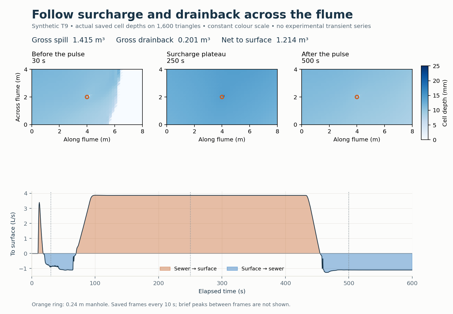
Synthetic T9 depth maps and exchange hydrograph

The three maps use actual saved cell depths and a common 0–25 mm colour scale. The orange ring marks the manhole. Constant surface inflow continues, so the plotted surface water includes both inflow and surcharge. The interactive viewer plays all 60 saved frames with a synchronised hydrograph cursor and gross spill/drainback totals. It also allows the steady comparison to be inspected by regime. It works offline and can export its plotted data. Saved depths are spaced 10 s apart; their 20.909 mm maximum omits brief peaks between frames. The all-step maximum is 24.803 mm. No measured transient hydrograph is implied.

Interpretation limits and further qualification

The law-only check scales the root regularisation head to 0.02/6 m, while the routed model retains 0.02 m, inside the rig's millimetre-scale head range. Wet-stencil head sampling is not the paper's average over all cells inside the opening. The nearest-centroid surface probe is displaced from the exact transducer location, and treating the remote pipe pressure as manhole head omits local losses. These are modelling limitations, not uncertainty removed by the published coefficient preset.

Experimental qualification requires measured transient pressure and exchange series, resolved routing-step and mesh convergence, acceptable separate and combined mass balances, and a reviewed representation of head sampling, regularisation and opening-footprint delivery. Any fit to the 36 steady rows must be labelled calibration and checked against independent measurements. The example supports inspecting the current implementation and its limits; it does not establish experimental validation of the coupled solver.

Reference: Rubinato, M., Martins, R., Kesserwani, G., Leandro, J., Djordjević, S., and Shucksmith, J. (2017). Experimental calibration and validation of sewer/surface flow exchange equations in steady and unsteady flow conditions. Journal of Hydrology 552, 421-432. doi:10.1016/j.jhydrol.2017.06.024. Reference tables: CC-BY-4.0; original numerical input decks: CC0-1.0.

Table of Contents