 |
OpenSWMM Engine
6.0.0-alpha.4
Data-oriented, plugin-extensible SWMM Engine (6.0.0-alpha.4)
|
|
OpenSWMM Engine
6.0.0-alpha.4
Data-oriented, plugin-extensible SWMM Engine (6.0.0-alpha.4)
|
______________________________________________________________________________
Chapters 3, 4 and 8 all solve one-dimensional flow along a conduit. When a sewer surcharges, the water that leaves the network spreads over the street, ponds behind a kerb, follows the terrain rather than the pipe, and re-enters the network somewhere else. Chapter 2's node-link model has no representation for any of that: SWMM 5 either discards the overflow or holds it in a fictitious ponded area above the node, to be returned to the same node later.
This chapter documents the optional two-dimensional overland-flow domain OpenSWMM provides for that water — a cell-centred finite-volume solver for the local-inertial shallow-water equations on an unstructured triangular mesh, coupled bidirectionally to the node-link network.
The module is activated by the presence of a mesh in the project ([2D_VERTICES] and [2D_TRIANGLES], inline or via [2D_MESH_FILE]) rather than by a routing option. IGNORE_2D YES disables it while leaving the mesh parsed and editable. The 1D network continues to route by whatever FLOW_ROUTING selects; the 2D domain supplements the network routing rather than replacing it.
A surface that is a domain in its own right. Ponded volume in the node-link model belongs to the node it came from. On the 2D mesh it belongs to the terrain: it flows downhill, splits at a crown, pools in a sag, and drains into whichever inlet it reaches. Which node receives the water is an outcome of the calculation rather than an input to it.
Flow paths the network does not contain. Overland routes — a road acting as a channel, flow over an embankment, a flow path between two otherwise unconnected catchments — exist in the terrain and nowhere in the pipe topology.
A flood extent. The depth field over a real surface is the quantity flood mapping needs. A ponded volume at a node is not one.
Several limitations should be noted. The method does not replace hydrology: unless RAINFALL_MODE says otherwise the mesh receives the same rainfall the subcatchments do, and both would deliver it (§9.8). It does not infiltrate — the mesh has no soil column, and water on it leaves only by flowing away, evaporating, or entering the network (§9.12). And its momentum equation is an approximation of the full shallow-water system: §9.2 states what is dropped and §9.10 measures what that costs.
Depth-averaged mass conservation over a surface of bed elevation \(z(x,y)\) and free surface \(\eta = z + h\), with unit-width discharge \(\mathbf{q} = h\mathbf{u}\) (m²/s):
\[\frac{\partial h}{\partial t} + \nabla \cdot \mathbf{q} = i - e + s\] | Continuity | (9-1) |
where \(i\) is rainfall intensity, \(e\) the evaporation rate and \(s\) the exchange with the 1D network, all as velocities normal to the surface.
The momentum equation solved is the local-inertial (or inertial-wave) approximation of Bates et al. (2010):
\[\frac{\partial \mathbf{q}}{\partial t} + g\,h\,\nabla\eta + \frac{g\,n^{2}\,\lvert\mathbf{q}\rvert\,\mathbf{q}}{h^{7/3}} = 0\] | Momentum | (9-2) |
with \(g = 9.80665\) m/s² and \(n\) Manning's roughness. Compared with the full shallow-water momentum equation, the **convective acceleration term \(\nabla\cdot(\mathbf{q}\mathbf{q}/h)\) is dropped**. Everything else — local acceleration, the pressure gradient written as a free-surface slope, and bed friction — is retained.
This is the single most consequential modelling decision in the chapter, and it is a deliberate one. Retaining \(\partial\mathbf{q}/\partial t\) is what separates (9-2) from the diffusive wave: the diffusive wave has no inertia at all, so a flood front on a flat surface propagates at a speed set by the numerical step rather than by the physics, and the scheme becomes stiff exactly where floods are shallow. Dropping the convective term is what separates (9-2) from the full system, and it costs the Bernoulli terms: the scheme cannot represent a drawdown over a crest, a stable hydraulic jump position, or a fully supercritical profile. §9.10 shows both effects measured against closed-form solutions.
The practical justification is that urban flood flows are dominated by gravity and friction. Bates et al. (2010) and de Almeida and Bates (2013) delimit the regime: the local-inertial approximation is accurate for subcritical flows over gentle slopes at Froude numbers below about 0.5, and degrades progressively as \(Fr \to 1\). Flow that is persistently supercritical, or where the momentum flux through a contraction sets the answer, is outside it.
For steep faces the model would accelerate without bound, since nothing in (9-2) limits the velocity a slope can generate. A Froude clamp supplies that limit numerically (§9.5.1).
Unlike the internal discretization of Chapter 8, the mesh is an explicit part of the model. Its cells appear in results, carry per-cell parameters, and are addressable by the API.
Cells are triangles, listed in [2D_TRIANGLES] by three vertex indices from [2D_VERTICES], with Manning's \(n\) and an optional initial depth per cell:
Bed elevation is carried at the vertices. A cell's centroid elevation \(z_c\) is the mean of its three vertex elevations, so the cell bed is the plane through them — a fact the closure of §9.4 uses directly. Nothing in the solver reads a cell-constant bed.
Edge–neighbour adjacency is built by hashing each triangle's three sorted vertex pairs: an edge claimed twice is interior and the two triangles become neighbours; an edge claimed once is a domain boundary and carries a boundary condition (§9.6). The convention throughout is that **local edge \(e\) is opposite vertex \(e\)**, so its endpoints are the triangle's other two vertices. Both incident cells of an interior edge therefore compute the same endpoint elevations, which is what makes the face depth of §9.5.2 antisymmetric and the flux conservative.
Interior edges are then enumerated once each as unique faces, with the left cell \(L\), the right cell \(R\), the edge length \(\xi\), the outward normal of \(L\)'s slot (which points \(L \to R\)), the edge midpoint, and the face-normal centroid separation
\[d_{n} = \max\left( \lvert (\mathbf{x}_{R} - \mathbf{x}_{L})\cdot\hat{\mathbf{n}} \rvert,\ 0.3\,\lvert \mathbf{x}_{R} - \mathbf{x}_{L}\rvert \right)\] | (9-3) |
The floor keeps a near-degenerate sliver — where the centroid chord is nearly parallel to the shared edge — from producing an unbounded surface slope. Face roughness is the mean of the two cells' \(n\).
Each cell also carries a characteristic length derived from the discrete operator rather than from geometry, for the time-step bound of §9.5.5:
\[L_{char} = \sqrt{\frac{2A}{\sum_{f} \xi_{f}/d_{n,f}}}\] | (9-4) |
A cell none of whose edges is an interior face has an empty sum in (9-4) and keeps the altitude proxy \(2A/\xi_{max}\) instead; such a cell carries no interior flux until a neighbouring face opens, so the proxy never governs a coupled update.
Every quantity above is planimetric. Areas, lengths and normals are computed in plan rather than on the sloped surface. On terrain steep enough for that distinction to matter the shallow-water equations are themselves the wrong model, so this is a consistent rather than an incidental choice.
Per-edge conveyance factors in \([0,1]\) may be attached with [2D_EDGE_CONVEYANCE], multiplying the flux across that edge — the transmissivity \(\psi\) of the integral-porosity shallow-water literature (Sanders et al., 2008; Bruwier et al., 2017), used to represent sub-grid obstructions such as walls and fences without meshing them. Values are mirrored onto both slots of an interior edge, so the restriction stays symmetric and the flux stays conservative.
Initial conditions come from INIT_DEPTH in [2D_TRIANGLES] (a depth in mesh units, converted to a cell volume through the closure of §9.4) and optionally [2D_INITIAL_VELOCITY], which seeds face momentum from the cell velocities. Without the latter a model can only start from rest, which excludes solutions such as Thacker's oscillating basins whose initial state has \(\mathbf{u} \neq 0\).
The conserved variable is cell volume \(V\) rather than depth. Depth follows as the cell-mean \(\bar{h} = V/A\). The closure is the relation that recovers a free-surface elevation \(\eta\) from that volume, and it is where a triangular mesh with sloping cell beds differs sharply from a raster of flat cells.
CELL_CLOSURE FLAT (the default) uses
\[\eta = z_{c} + \bar{h}\] | (9-5) |
which is exact for a fully wetted cell and wrong for a partially wet one. On a cell whose bed spans a slope or a step, spreading the water uniformly over the whole cell raises the computed surface above the true waterline — by up to two-thirds of the cell's relief. That error is a head, and a head drives flux: the classic symptom is thin films creeping uphill at a shoreline, and a lake at rest that is not a steady state where it meets the bank.
CELL_CLOSURE VFR uses the exact stage–storage relation of the plane bed through the cell's three vertex elevations — the volume/free-surface relationships of Begnudelli and Sanders (2006, 2007). With sorted elevations \(z_1 \le z_2 \le z_3\) and \(\bar{z} = (z_1+z_2+z_3)/3\):
\[\bar{h}(\eta) = \frac{(\eta - z_{1})^{3}}{3(z_{2}-z_{1})(z_{3}-z_{1})}\] | \(z_{1} < \eta \le z_{2}\) | (9-6a) | |
\[\bar{h}(\eta) = (\eta - \bar{z}) + \frac{(z_{3}-\eta)^{3}}{3(z_{3}-z_{1})(z_{3}-z_{2})}\] | \(z_{2} < \eta \le z_{3}\) | (9-6b) | |
\[\bar{h}(\eta) = \eta - \bar{z}\] | \(\eta \ge z_{3}\) | (9-6c) |
The solver needs the inverse \(\eta(\bar{h})\). On the lower branch it is a closed-form cube root; on the upper branch a safeguarded Newton iteration bracketed by \([z_2, z_3]\), which converges unconditionally because \(d\bar{h}/d\eta = A_{wet}/A > 0\) there. Note that (9-6c) is identical to the flat closure (9-5), since \(z_c = \bar{z}\) — the two closures differ only on partially wet cells, which is precisely the claim.
As a cell dries, \(d\eta/dV = 1/A_{wet}\) diverges. VFR_MIN_WET_FRAC ( \(\varepsilon\), default 0.01) bounds it by continuing the exact relation below wetted fraction \(\varepsilon\) along its tangent line, keeping the closure \(C^1\) and monotone with \(d\eta/dV \le 1/(\varepsilon A)\). The regularized forward and inverse relations are exact inverses of each other for the same \(\varepsilon\), so seeding a state from heads and reading it back as volumes round-trips.
VFR is correct and is not the default. It restores the C-property at shorelines and removes the uphill-creep artifact, but in doing so it resolves a wetting and drying front that the flat closure freezes out — measured at three to eight times more solver substeps. For deep urban flooding, where partially wet cells are a thin fringe around a large wetted area, the flat closure is both faster and adequate. For shallow sheet flow on gentle slopes, where most cells are partially wet, VFR is the right choice and the cost is the price of the answer. Pair it with FACE_RECONSTRUCTION VFR_FACE (§9.5.2); the two halves address the same artifact from the cell side and the face side.
The relations (9-6) are evaluated by a single header-only routine shared by the serial marcher, the boundary path and the GPU kernels, so every backend reconstructs the identical surface. Three auxiliary quantities appear. The wetted-area fraction of the planar bed — which is also \(d\bar{h}/d\eta\) — with sorted elevations \(z_1 \le z_2 \le z_3\) and relief \(R = z_3 - z_1\):
\[w(\eta) = \frac{(\eta - z_{1})^{2}}{(z_{2}-z_{1})\,R}\] | \(z_{1} < \eta \le z_{2}\) | (9-20a) | |
\[w(\eta) = 1 - \frac{(z_{3} - \eta)^{2}}{R\,(z_{3}-z_{2})}\] | \(z_{2} < \eta < z_{3}\) | (9-20b) |
with \(w = 0\) below \(z_1\) and \(w = 1\) above \(z_3\). The stage at which the wetted fraction equals the regularization floor \(\varepsilon\):
\[\eta_{s} = z_{1} + \sqrt{\varepsilon\,(z_{2}-z_{1})\,R}\] | \(\varepsilon \le (z_{2}-z_{1})/R\) | (9-21a) | |
\[\eta_{s} = z_{3} - \sqrt{(1-\varepsilon)\,R\,(z_{3}-z_{2})}\] | otherwise | (9-21b) |
Below the switch depth \(\bar{h}_s = \bar{h}(\eta_s)\) from (9-6) the inverse continues along the tangent line,
\[\eta(\bar{h}) = \eta_{s} - \frac{\bar{h}_{s} - \bar{h}}{\varepsilon}\] | \(\bar{h} \le \bar{h}_{s}\) | (9-22) |
and on the lower branch it is closed-form,
\[\eta = z_{1} + \left\lbrack 3\,\bar{h}\,(z_{2}-z_{1})\,R \right\rbrack^{1/3}\] | \(\bar{h} \le (z_{2}-z_{1})^{2}/(3R)\) | (9-23) |
The inverse \(\eta(V)\) is evaluated by the following case ladder, in this order:
The forward relation \(\bar{h}(\eta)\) applies the same regularization — exact above \(\eta_s\), the tangent below, floored at zero — so forward and inverse are exact inverses for the same \(\varepsilon\) and head-seeded and volume-seeded states round-trip. A dry cell's head under VFR is seeded at \(\eta(0) = \eta_s - \bar{h}_s/\varepsilon \in (z_1, \eta_s)\), the value the closure itself returns at \(V = 0\), so that seeding the head back through the forward relation reproduces exactly zero volume. Figure 9-2 (§9.5.9) sketches the wetting cases.
Implementation: the closure lives in src/engine/2d/mesh/VfrClosure.hpp — openswmm::twoD::vfrSort3, openswmm::twoD::vfrWetFraction, openswmm::twoD::vfrStageAtWetFraction, openswmm::twoD::vfrMeanDepthFromEtaExact, openswmm::twoD::vfrMeanDepthFromEta, openswmm::twoD::vfrEtaFromMeanDepth and openswmm::twoD::vfrDryEta. The solver enters through openswmm::twoD::inertial::etaDepthScalar and openswmm::twoD::inertial::volumeFromEtaScalar in src/engine/2d/solver/InertialKernels.hpp, whose FLAT branch is (9-5); the flat-relief guard is kVfrFlatRelief ( \(10^{-9}\) m).
The discretization is a cell-centred finite-volume method with a staggered face variable: cells hold volume, faces hold the unit-width discharge \(q\) normal to the face, positive from \(L\) to \(R\). Time integration is explicit, with per-cell local time stepping.
Each face integrates (9-2) along its own normal over its own step \(\Delta t_f\):
\[q^{n+1} = \frac{\hat{q} - g\,h_{f}\,\Delta t_{f}\,S}{1 + g\,\Delta t_{f}\,n_{f}^{2}\,\lvert\mathbf{q}_{f}\rvert / h_{f}^{7/3}}\] | (9-7) |
with the free-surface slope
\[S = \frac{\eta_{R} - \eta_{L}}{d_{n}}\] | (9-8) |
Three details in (9-7) carry weight.
Friction is semi-implicit. Writing the friction term with \(q^{n+1}\) in the numerator and \(\lvert\mathbf{q}\rvert\) from the previous state puts it in the denominator, which is unconditionally stable: however large the friction coefficient, the update can only shrink \(q\) towards zero, never overshoot through it. An explicit friction term would impose a step limit that scales as \(h^{7/3}/n^{2}\) — unusable on thin films, which is where most of the cells are.
The friction magnitude is taken from the flow vector rather than the face-normal component. Manning friction acting on the normal component is \(n^{2} q_{n} \lvert\mathbf{q}\rvert / h^{7/3}\). Using \(\lvert q_n \rvert\) instead makes the damping a face applies depend on the face's orientation relative to the flow — a face at 45° to a uniform sheet under-damps by \(\sqrt{2}\) — so no smooth surface can satisfy every face of a triangulated slope simultaneously, and the steady state corrugates cell to cell. The vector at the face is the mean of the two incident cells' Perot-reconstructed discharge vectors (§9.5.4, Eq. 9-16), and its magnitude is floored at the face's own discharge:
\[\lvert\mathbf{q}_{f}\rvert = \max\!\left( \lvert q_{f} \rvert,\ \left\lvert \tfrac{1}{2}(\mathbf{q}_{L} + \mathbf{q}_{R}) \right\rvert \right)\] | (9-24) |
so a face whose cell reconstruction lags its own discharge — the first firing after a front arrives, or immediately after activation — never under-damps. With \(\theta = 1\) the cell discharge vectors are not allocated at all: the update uses \(\hat{q} = q_f\) and \(\lvert\mathbf{q}_f\rvert = \lvert q_f \rvert\), recovering the original Bates et al. (2010) scheme exactly. The friction exponent is evaluated as \(h^{7/3} = h^{2}\sqrt[3]{h}\) rather than through pow().
** \(\hat{q}\) is a lateral average, not \(q\) itself.** With THETA \(= \theta\),
\[\hat{q} = \theta\,q_{f} + (1-\theta)\,\tfrac{1}{2}\left( \mathbf{q}_{L} + \mathbf{q}_{R} \right)\cdot\hat{\mathbf{n}}\] | (9-9) |
\(\theta = 1\) recovers the original Bates et al. (2010) scheme, which carries no numerical diffusion and is prone to a checkerboard oscillation in thin films on steep faces. \(\theta < 1\) blends in the neighbouring cells' reconstructed discharge and damps it — the weighted formulation of de Almeida et al. (2012). The default \(\theta = 0.8\) applies enough diffusion to suppress the oscillation without visibly smearing fronts.
Finally the result is clamped:
\[\lvert q^{n+1} \rvert \le Fr_{max}\,h_{f}\sqrt{g\,h_{f}}\] | (9-10) |
FROUDE_MAX defaults to 1.5. This is the steep-face guard: with no convective term there is nothing in (9-2) to arrest acceleration down a steep face, so the supercritical limit must be imposed rather than resolved. Raising it lets genuinely transcritical cases run (§9.10) at the cost of the guard.
As coded, one face firing over its step \(\Delta t_f\) proceeds in a fixed order: (i) evaluate the face depth (§9.5.2) and wall the face if \(h_f \le\) DRY_DEPTH, zeroing its momentum; (ii) form \(\hat{q}\) by (9-9) and the friction magnitude by (9-24); (iii) zero the free-surface difference if it lies below the \(10^{-12}\) m deadband (§9.5.3) and form the slope (9-8); (iv) apply (9-7) and then the clamp (9-10); (v) rescale by the positivity share (9-15) where it binds; (vi) book \(\pm\Delta M\) by (9-13). The stored face discharge is the post-clamp, post-rescale value, so the momentum a face carries always matches the mass it moved.
The depth in (9-7) is a property of the face, and how it is defined decides when water is allowed to cross. Under FACE_RECONSTRUCTION MEAN (the default):
\[h_{f} = \max(\eta_{L}, \eta_{R}) - \max(z_{c,L}, z_{c,R})\] | (9-11) |
\(h_f \le\) DRY_DEPTH makes the face a wall for that substep and its momentum is zeroed. This is the standard "flow depth above the higher
bed" rule, and it is what makes the scheme handle wetting and drying without regime-switching logic — but its bed is the higher centroid elevation. A thin crest resolved as a line of high vertices — a levee, a kerb, a road crown — has its height diluted by roughly a third when averaged into the flanking centroids, so water crosses it before it reaches it.
FACE_RECONSTRUCTION VFR_FACE uses instead the exact mean depth of the driving surface over the wetted portion of the shared edge, evaluated against the edge's true endpoint elevations \(z_{lo} \le z_{hi}\) (Begnudelli and Sanders, 2007, Eq. 14):
\[h_{f} = 0\] | \(\eta \le z_{lo}\) | (9-12a) | |
\[h_{f} = \frac{(\eta - z_{lo})^{2}}{2(z_{hi}-z_{lo})}\] | \(z_{lo} < \eta \le z_{hi}\) | (9-12b) | |
\[h_{f} = \eta - \tfrac{1}{2}(z_{lo}+z_{hi})\] | \(\eta > z_{hi}\) | (9-12c) |
with \(\eta = \max(\eta_L, \eta_R)\). The quadratic branch matches value and slope at both joins, so overtopping onset is \(C^1\) and the flux does not jump when the waterline crosses the edge. The gate (9-12a) is the substantive part: a cell holding water pooled below the whole shared edge conveys nothing across it. Embankments hold to their real crest, and drainage no longer strands water on slopes.
Both branches are single-sourced and used identically by the interior faces, the boundary edges and the GPU kernels, so all backends agree.
A body of water at rest over arbitrary bathymetry must stay at rest. This is the C-property, and it is not automatic — a scheme that discretizes the bed slope and the pressure gradient separately will generally produce a spurious flux from their imbalance.
Writing the pressure gradient as the free-surface slope (9-8) makes the property structural: at rest \(\eta_L = \eta_R\), so \(S = 0\) exactly, and (9-7) with \(\hat{q} = q = 0\) returns zero for any bed whatsoever. Likewise a dry neighbour standing higher gives \(h_f \le 0\) and the face is a wall — there is no uphill creep to suppress.
One numerical guard is needed. The closure round-trip \(V \to \eta\) introduces rounding noise of order 1 ulp, and the square-root character of the friction balance amplifies it: a persistent \(\Delta\eta \sim 10^{-16}\) m sustains \(q \sim 10^{-6}\) m²/s. A slope below \(10^{-12}\) m is therefore set to exactly zero, far below any physical head, after which the friction denominator decays \(q\) geometrically and rest states are exact rather than merely small. §9.10 measures the result at \(10^{-16}\) relative error on the SWASHES lake-at-rest cases.
A face firing books the identical volume transfer into a per-side accumulator:
\[\Delta M = q^{n+1}\,\xi\,\Delta t_{f}, \qquad \text{acc}_{L} \mathrel{-}= \Delta M, \quad \text{acc}_{R} \mathrel{+}= \Delta M\] | (9-13) |
and a cell firing gathers and clears its own side of each incident accumulator:
\[V^{n+1} = V^{n} + \sum_{f} \text{acc}_{f,i} + \Delta t_{c}\,A\,(i - e + s)\] | (9-14) |
after which \(\eta\) and \(\bar{h}\) are recomputed through the closure of §9.4. Because the two sides of a face are written from the same floating-point product, conservation is exact by construction rather than to within a tolerance — including across a local-time-stepping tier interface, where the two sides apply their halves at different times (§9.5.6). The sum of cell volumes plus pending accumulators is an invariant of the face phase, and the engine can assert it directly (OPENSWMM_2D_MARCHER_CHECK).
Positivity is enforced at face cadence rather than by a post-hoc clamp. A cell has at most three outgoing faces, so capping each exporting face at a share \(\beta/3\) of its exporting cell's volume bounds the total export at \(\beta V\) per cell step without any cross-face coordination:
\[\lvert q^{n+1}\rvert\,\xi\,\Delta t_{f} \le \frac{\beta}{3}\,\frac{V_{exp}}{2^{\,k_{exp} - k_{f}}}\] | (9-15) |
\(\beta\) is exchange_beta (0.8). The tier ratio in the denominator matters: an exporting cell republishes its volume only at its own firings, and a finer face fires \(2^{k_{exp}-k_f}\) times in between, so without dividing the share the repeated takes drain the cell. When a face is rescaled, the same rescaled flux updates both sides, so the cap costs nothing in conservation. A zero floor at the cell update remains as a backstop; with the face caps in place it does not engage.
The cell's discharge vector — needed for the friction magnitude and the \(\theta\) blend — is reconstructed at the cell's own cadence from its face fluxes by the Perot (2000) formula:
\[\mathbf{q}_{i} = \frac{1}{A_{i}}\sum_{f} s_{f}\,q_{f}\,\xi_{f}\,\left( \mathbf{x}_{f} - \mathbf{x}_{i} \right)\] | (9-16) |
with \(s_f = \pm 1\) the outward orientation of face \(f\) for cell \(i\) and \(\mathbf{x}_f\) the edge midpoint.
Each cell's stable step follows from the gravity-wave celerity and its own characteristic length:
\[\Delta t_{i} = \alpha \frac{L_{char,i}}{\sqrt{g h_{i}} + \lvert \mathbf{u}_{i}\rvert}\] | (9-17) |
with \(\alpha =\) CFL_NUMBER, default 0.7, and the base step of a macro cycle \(\Delta t_0 = \min_i \Delta t_i\), further capped by MAX_TIMESTEP. Only active cells wetter than DRY_DEPTH enter the census — a film the solver will not move imposes no constraint — and a fully quiescent active set falls back to \(\Delta t_0 =\) MAX_TIMESTEP. The advective augmentation \(\lvert\mathbf{u}_i\rvert = \lvert\mathbf{q}_i\rvert/h_i\) is evaluated from the Perot vector when the depth exceeds \(10^{-6}\) m and \(\theta < 1\), and taken as zero otherwise.
\(L_{char}\) is the operator-derived length of (9-4) rather than a geometric proxy, and the difference matters. The face update couples cells through \(g h \xi_f/(A\,d_{n,f})\); the worst (odd–even) mode of that operator has eigenvalue \(\lambda = 2(gh/A)\sum_f \xi_f/d_{n,f}\), and the explicit update is linearly stable for \(\Delta t \le 2/\sqrt{\lambda}\), which is exactly (9-4) divided by the celerity. Defining \(L_{char}\) this way makes \(\alpha\) a true Courant fraction: \(\alpha = 1\) is the linear stability limit on any mesh, and the default 0.7 is a uniform 30 % margin. A raster of squares recovers the classical \(c\,\Delta t/\Delta x \le 1/\sqrt{2}\); a union-jack pair of right triangles gets \(0.408\,\Delta x\). The obvious geometric proxy \(2A/\xi_{max}\) returns \(0.707\,\Delta x\) on that same union-jack mesh — an overstatement by \(\sqrt{3}\), and the reason frictionless basins seiched at nominal Courant numbers that looked conservative.
Between full rebuilds the tier lists are frozen while depths keep evolving, so \(\Delta t_0\) is re-minimized every macro cycle. It may be tightened at any time — every tier still satisfies \(\Delta t_i \ge 2^{k}\Delta t_0\) — but growing it requires reassigning tiers and therefore waits for a rebuild.
A flood mesh is heterogeneous by nature: a 0.5 m cell at a coupled manhole and a 20 m cell on a floodplain differ by two orders of magnitude in stable step. Marching the whole mesh at the smallest one wastes almost all of the work.
The solver instead assigns each cell a power-of-two tier \(k\) from the ratio \(\Delta t_i/\Delta t_0\), capped at LTS_TIERS (default 4, allowing an 8× spread; up to 8 tiers, 128×). A macro cycle is \(2^{K-1}\) base substeps; tier \(k\) fires every \(2^{k}\) substeps with \(\Delta t = 2^{k}\Delta t_0\). Within a substep all due faces fire first, then all due cells — faces read the surfaces their incident cells published at those cells' last firings.
A face belongs to the finer of its two incident cells' tiers. It therefore always integrates at the rate the sharper side needs, reading the coarser side's surface frozen since that cell last fired. This is what makes tier interfaces safe without interpolation, and (9-13) is what makes them conservative: the same \(\pm\Delta M\) is booked once and applied by each side at its own firing.
Cells whose forcing changes at the fastest cadence are pinned to tier 0 regardless of their Courant number — boundary cells and cells carrying a 1D coupling point. For these cells the forcing, rather than the celerity, sets the resolution requirement.
Most of a rain-on-grid mesh is not flowing. A cell is flux-active only above H_MOVE (default 3 mm), with hysteresis: entering cells need \(h_{move} + \delta\), active cells stay until \(h_{move} - \delta\), where \(\delta = \min(1\ \text{mm},\ h_{move}/2)\). Scaling the band with H_MOVE matters on shallow benchmarks — a fixed ±1 mm band made H_MOVE \(= 10^{-4}\) require 1.1 mm to activate, ten times the requested threshold, which freezes wetting fronts in place.
Two rules complete the set. A face flows only when both incident cells are active — a one-sided face would export volume into a cell whose update never runs, and measured as an 18 % basin loss when it was allowed. A one-ring halo around the active set therefore guarantees an advancing front always has an active receiving cell.
Inactive cells are not skipped, they are integrated lazily: rainfall and held coupling accumulate as pure storage over the whole interval since the last synchronization, in one pass, because a cell below H_MOVE has no face flux by construction. This is what makes rain-on-grid over a large dry mesh nearly free. A rainfall rate as such never activates a cell — activation follows only from the accumulated depth crossing the threshold at a rebuild, which is the point of the lazy tier — whereas a nonzero coupling flux activates its cell immediately, as do the pinned boundary and coupling-point cells of §9.5.6.
The active set and the tier assignment are rebuilt every four macro cycles rather than every substep; the cost of the rebuild is \(O(n_{cells})\) and dominated everything else when it ran per routing step on a large mesh.
The solver's working set is three structure-of-arrays blocks, sized once at initialization.
Per unique interior face (built by the edge enumeration of §9.3): the incident cells \(c_L < c_R\); the edge length \(\xi\); the unit normal \(\hat{\mathbf{n}}\) oriented \(L \to R\) and the edge midpoint; the reciprocal face-normal centroid separation \(1/d_n\) of (9-3); the squared face roughness \(n_f^2 = \left(\tfrac{1}{2}(n_L + n_R)\right)^2\); the sorted true endpoint bed elevations \(z_{lo} \le z_{hi}\) of the shared edge (for VFR_FACE); and the two flat edge-slot indices \(3t + e\) used to publish fluxes back into the per-cell edge arrays. The prognostic state per face is the discharge \(q\) and the two pending-transfer accumulators \(\text{acc}_L\), \(\text{acc}_R\) of (9-13), plus a face tier.
Per cell: the conserved volume \(V\) and the reconstructed \(\eta\) and \(\bar{h}\); the source rates (rainfall, evaporation demand, coupling flux, all m/s); the Perot discharge vector \((q_{cx}, q_{cy})\), allocated only when \(\theta < 1\); the characteristic length \(L_{char}\) of (9-4); the tier, the active flag and the tier-0 pin flag; and a CSR incidence — for cell \(i\) the incident unique faces with orientation signs \(\pm 1\) — so the continuity gather is a race-free per-cell loop.
Per vertex: coordinates and bed elevation, plus the reconstruction stencils of §9.9. Per flat edge slot: the published volumetric flux and the boundary-condition tables of §9.6.
One solver advance over a window \([t,\ t + \Delta t]\) executes:
The face and cell passes are OpenMP-parallel with static scheduling and the project's THREADS setting. Each face is written by exactly one iteration and touches only its own accumulator slots, and each cell gathers only its own accumulator sides, so both passes are race-free and bit-identical to serial execution for any thread count. The boundary and coupling loops are serial; they are perimeter- and point-count-sized. The quantity \(\sum_i V_i + \sum_f (\text{acc}_{L,f} + \text{acc}_{R,f})\) is invariant under the face phase and is asserted directly when OPENSWMM_2D_MARCHER_CHECK is set.
Figure 9-1 assembles the co-advance batch of §9.7.3 and the marcher's substep loop into one workflow.
flowchart TD
    A[1D routing step completes - node heads current] --> B{Pending span reaches the sync batch}
    B -- no --> A
    B -- yes --> C[Save state and seed withdrawal budgets]
    C --> D[Accumulate outfall discharge and inject as batch-rate source]
    D --> E[Refresh rainfall, forcing overrides and boundary values]
    E --> F[Marcher advance over the batch span]
    F --> G{Rebuild due}
    G -- yes --> H[Settle accumulators, lazy sources, active set, tiers, dt0]
    G -- no --> I[Tighten dt0 from live depths]
    H --> J[Macro cycle of base substeps]
    I --> J
    J --> K[Fire due faces - depth, blend, update, clamp, positivity, book dM]
    K --> L[Fire due cells - gather, sources, closure, Perot]
    L --> M[Tier-0 firings - boundary edges and live junction exchange]
    M --> N{Batch span filled}
    N -- no --> G
    N -- yes --> O[Book junction, outfall and boundary ledgers into the 2D mass balance]
    O --> P[Queue exchange volumes for uniform delivery to 1D lateral inflow]
    P --> Q[Clear one-shot forcings, reset window accumulators]
    Q --> A
Figure 9-1 One 1D–2D co-advance batch and the explicit marcher's substep loop within it (rendered diagram)
Implementation: openswmm::twoD::ExplicitInertialSolver::advance drives the loop; openswmm::twoD::ExplicitInertialSolver::fireFaces, openswmm::twoD::ExplicitInertialSolver::fireCells, openswmm::twoD::ExplicitInertialSolver::syncAndRebuild, openswmm::twoD::ExplicitInertialSolver::settleAccumulators and openswmm::twoD::ExplicitInertialSolver::refreshDt0 implement the numbered steps. The face layout and CSR incidence are built by openswmm::twoD::InertialEdges::build (src/engine/2d/solver/InertialEdges.cpp); the scalar kernels live in src/engine/2d/solver/InertialKernels.hpp; the cell state arrays are openswmm::twoD::SurfaceStateData (src/engine/2d/data/SurfaceStateData.hpp).
The scheme has no regime-switching logic; wetting and drying emerge from a small set of thresholds applied uniformly. Table 9-1 collects them.
| Constant | Value | Origin | Role |
|---|---|---|---|
DRY_DEPTH | 0.001 m | [2D_OPTIONS] | Face-wall depth, friction depth floor, evaporation taper scale, coupling ramp scale, CFL census cutoff |
H_MOVE | 0.003 m | [2D_OPTIONS] | Flux-activation depth |
| \(\delta\) | \(\min(0.001\ \text{m},\ h_{move}/2)\) | derived | Activation hysteresis half-band |
| \(\varepsilon\) | 0.01 | VFR_MIN_WET_FRAC | Wetted-fraction floor of the VFR closure |
| slope deadband | \(10^{-12}\) m | fixed | Free-surface differences treated as exactly zero |
| flat-relief guard | \(10^{-9}\) m | fixed | Cell or edge relief below which the geometry is flat |
| \(\beta\) | 0.8 | fixed | Positivity and exchange availability fraction |
| rebuild cadence | 4 macro cycles | fixed | Active-set and tier refresh period |
Table 9-1 Wetting and drying thresholds and guards of the 2D solver (SI units)
The face-wet criterion. A face conveys only when its flow depth exceeds DRY_DEPTH: under MEAN the depth (9-11), under VFR_FACE the wetted-edge depth (9-12) of the driving surface over the edge's true endpoint beds. A face that fails the test is a wall for that substep and its momentum is set to exactly zero — walls carry no stale discharge into their next wet substep. A face also requires both incident cells active (§9.5.7); faces bordering an inactive cell have their momentum zeroed at the rebuild.
How a dry cell wets. The activation thresholds carry hysteresis,
\[h_{on} = h_{move} + \delta, \qquad h_{off} = \max(0,\ h_{move} - \delta), \qquad \delta = \min(0.001,\ h_{move}/2)\] | (9-25) |
entering cells needing \(h_{on}\) and active cells persisting to \(h_{off}\). A dry cell gains water in one of three ways. Distributed sources (rainfall) accumulate lazily as pure storage; the cell joins the active set at the first rebuild whose census finds its depth at or above \(h_{on}\). A concentrated source — a nonzero coupling flux — activates the cell at the next rebuild regardless of depth, as does membership in the pinned set. A neighbouring active cell activates it through the one-ring halo, after which the shared face joins the face lists; the first term to act on the newly wet cell is then the mass transfer (9-13), driven by the slope term of (9-7) integrated from \(q = 0\) — the friction denominator is near unity at \(q = 0\), so the initial specific discharge after one face step is \(-g\,h_f\,\Delta t_f\,S\).
How a front advances. Between rebuilds the active set is frozen, so a wetting front can cross at most one cell ring per rebuild period (four macro cycles). This is not a practical restriction: a fast front implies a small \(\Delta t_0\) through (9-17), so the rebuild period shrinks with the front's own time scale, and the halo guarantees the front always finds an active receiving cell — a one-sided face is never allowed to fire (§9.5.7).
Shorelines and the lake at rest. A dry neighbour standing higher gives \(h_f \le 0\) under (9-11) and the face is a wall — there is no uphill creep to suppress. Under the VFR closure the partially wet shoreline cell's \(\eta\) is exact rather than biased high (§9.4), and under VFR_FACE the gate (9-12a) blocks conveyance across any edge whose low point stands above the driving surface, so an emerged bump holds a lake at rest exactly. The \(10^{-12}\) m slope deadband removes the closure round-trip noise that would otherwise sustain a \(\sim 10^{-6}\) m²/s residual discharge (§9.5.3); the emerged-bump verification case of §9.10 measures the combined result at \(1.4 \times 10^{-16}\) relative depth error.
Draining and positivity. Every exporting face is capped at the tier-scaled \(\beta/3\) share of its exporting cell's volume, Eq. (9-15), so a cell's at most three outgoing faces can remove at most \(\beta V\) per cell step with no cross-face coordination. Boundary edges and the coupling exchange clamp in volume space — the applied change is recomputed after flooring the provisional volume at zero, so booking matches application exactly. The cell update keeps a plain zero floor as a backstop; with the caps in place it does not engage (a debug build with OPENSWMM_2D_MARCHER_CHECK reports any clamp below \(-10^{-12}\) m³).
The friction depth floor. No separate floor exists: the face-wall test guarantees \(h_f >\) DRY_DEPTH \(= 1\) mm before (9-7) is evaluated, so \(h_f^{7/3} \ge 10^{-7}\) m \(^{7/3}\) and the semi-implicit denominator is always finite. Because friction enters only through the denominator, it can shrink \(q\) toward zero and never reverse it.
Rain and evaporation on dry cells. The evaporation sink is the demand rate tapered by a cubic Hermite ramp below DRY_DEPTH,
\[e_{eff} = e \cdot \sigma\!\left( h/h_{dry} \right), \qquad \sigma(t) = \min(1, t)^{2}\left( 3 - 2\min(1, t) \right)\] | (9-26) |
with \(e_{eff} = 0\) for \(h \le 0\) or \(e \le 0\) — a drying cell cannot evaporate more water than it holds, and negative demand is treated as zero rather than as a condensation source. Rainfall on an inactive cell integrates in a single lazy pass over the whole interval since the last synchronization; the result is floored at zero volume, so a forced evaporation override on a dry cell is harmless.
Figure 9-2 sketches the geometry the rules act on: the three wetting cases of the planar-bed cell (§9.4.1) and the wetted-edge face gate (§9.5.2).
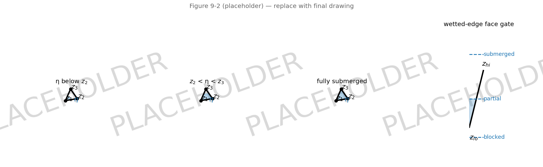
Figure 9-2 Wetting cases of a planar-bed triangular cell and the wetted-edge face gate (placeholder — to be replaced by a final drawing)
Implementation: the face-wet tests are openswmm::twoD::inertial::faceFlowDepth and openswmm::twoD::inertial::faceFlowDepthVfr over openswmm::twoD::inertial::faceDepthFromEta; the positivity share is applied in openswmm::twoD::ExplicitInertialSolver::fireFaces with the scale factor of openswmm::twoD::inertial::positivityScale; the hysteretic activation, halo and lazy source passes are openswmm::twoD::ExplicitInertialSolver::syncAndRebuild and openswmm::twoD::ExplicitInertialSolver::lazySourcesOnly; the evaporation taper is openswmm::twoD::evapSink (src/engine/2d/solver/SurfaceFluxCalculator.hpp). The slope deadband is kEtaDeadband in src/engine/2d/solver/InertialKernels.hpp.
Boundary edges — those claimed by only one triangle — default to no-flux walls. [2D_BOUNDARY_CONDITIONS] assigns any of five types per edge:
| Type | Parameter | Meaning |
|---|---|---|
WALL | — | Zero flux (default) |
NORMAL_FLOW | bed slope \(S\) | Manning outflow \(q = h^{5/3}\sqrt{S}/n\) per metre of edge |
SPECIFIED_STAGE / TS_STAGE | head, or time series | Prescribed free-surface elevation |
SPECIFIED_FLOW / TS_FLOW | discharge per metre, or time series | Prescribed unit discharge, outward positive |
RATING_CURVE | curve name | Stage → unit discharge lookup, resolved each step from the boundary cell's stage |
Time series and curve names are resolved to registry indices once, on the first advance, and evaluated every routing step thereafter. Prescribed stages share the mesh's vertical datum and prescribed flows the project's flow units, so both are converted to SI on the same terms as the mesh itself (§9.7.4).
A stage boundary is integrated with the interior momentum law, not with a conductance. The ghost state holds \(\eta = \eta_{bc}\) with a zero-gradient discharge, sitting across the edge at the centroid-to-edge distance \(2A/(3L)\), and (9-7) is applied to it exactly as to an interior face. The earlier treatment — a collapsed Manning flux toward the prescribed stage — was a diffusive-wave law grafted onto an inertial interior, and it showed: its conductance saturated the equilibrium clamp into a Dirichlet cell, and every boundary-driven steady case floated one head jump, of order \(v^{2}/2g\), above the stage it had been given. The bump cases of §9.10 pass because of this change.
A per-substep equilibrium clamp remains as a backstop: one substep may move a cell at most to the prescribed stage, never past it. At the inertial law's gravity-scale fluxes it rarely binds; on a tiny cell it prevents overshoot. Exchange is clamped in volume space and the booked flux re-derived from the applied change, so what is reported is exactly what was applied.
Cumulative boundary volume is tracked per edge, outward positive, and enters the 2D mass balance of §9.9.
Coupling is bidirectional and mass-conservative, and it is where a 2D module earns or loses its credibility. Two mechanisms exist, one for junctions and one for outfalls.
[2D_VERTEX_NODE_MAP] and [2D_TRIANGLE_NODE_MAP] associate a mesh vertex or cell with a SWMM node, with a discharge coefficient \(C_d\) (default 0.65) and an exchange area. Exchange is an orifice law on the head difference:
\[Q = C_{d}\,A_{eff}\,\mathrm{sign}(\Delta h)\,\sqrt{2g}\ \varphi\!\left(\lvert\Delta h\rvert\right), \qquad \Delta h = h_{2D} - h_{1D}\] | (9-18) |
positive draining the surface into the network. Three regularizations turn (9-18) from a stiffness source into something an explicit solver can integrate:
A bounded square root. \(dQ/d\Delta h \to \infty\) as \(\Delta h \to 0\) is exactly the regime a fill-and-spill manhole hovers in. Below 2 cm, \(\varphi\) is a \(C^1\) quadratic matching \(\sqrt{x}\) in value and slope at the join and having finite slope at zero.
A capped-pipe gate. A manhole with its lid on exchanges through the network only when the higher of the two heads reaches the crown elevation \(z_{inv} + D_{full}\). A Hermite smoothstep over a 5 cm band above the crown opens the exchange, and the effective area transitions smoothly from the inlet area to twice it over the same scale as the node surcharges.
Source-side wet/dry ramps. \(Q\) is multiplied by a smoothstep on the source side's depth relative to DRY_DEPTH, so a drain self-limits to zero as the cell empties and a spill self-limits as the node empties. This replaces a held-flux availability cap and is what makes the exchange stable inside the solver's inner loop rather than only across a window.
The exchange is evaluated live, at tier-0 cadence, against the current 2D heads and the routing step's 1D heads, and \(\int Q\,dt\) is accumulated exactly per point. Two hard caps make the ledger unfalsifiable: a drain may take at most \(\beta\) of the source cell's volume per substep, and a spill draws against a per-node budget of the node's stored volume for the whole advance — so the same water cannot spill twice within a routing step.
The 2D head at a coupling point is not simply a cell head. Vertex-coupled points use a wet-masked, depth-weighted mean of the incident cells' free surfaces under the VFR closure: a manhole vertex is commonly carved below the surrounding terrain, and a geometric average over incident cells would read dry-cell bed elevations as a water surface and pin the exchange at a phantom head from the first step.
Under dynamic wave routing the exchange would otherwise be a zero-sensitivity explicit source in the node continuity equation, which churns the Picard iteration. The head sensitivity
\[G = -\frac{\partial Q}{\partial h_{1D}} = C_{d}A_{eff}\sqrt{2g}\ \varphi'\!\left(\lvert\Delta h\rvert\right)\cdot(\text{gate})\cdot(\text{ramp}) \ \ge\ 0\] | (9-19) |
is scattered into the node's \(\sum dQ/dH\) denominator each iteration. The gate and ramp derivatives are deliberately dropped so the term can only be positive — a pure damping contribution, never a destabilizing one.
Exchange volumes reach the 1D side through the lateral-inflow delivery queue, drained at a uniform rate over the batch span rather than as a single-step pulse.
An outfall coupled to the mesh works in both directions.
Outward, the node's net discharge for the routing step is accumulated and injected into the 2D cells as a constant-rate source over the subcycle. Withdrawals — a submerged outfall drawing surface water back into the pipe — are capped by a per-cell budget seeded from the state the batch started from, so a batch's cumulative withdrawal can never overdraw it.
Inward, the 2D surface acts as dynamic tailwater. The 2D stage at the coupling point is cached, and the outfall's boundary condition becomes \(\max(h_{standard}, h_{2D})\), applied inside the dynamic-wave iteration so it survives every Picard pass. Flap gates are honoured: the gate decision is made where the current \(h_{standard}\) is visible.
The wet/dry gate here is keyed on depth in excess of DRY_DEPTH, not on depth. The reason is specific: a draining cell comes to rest at a film at or just below DRY_DEPTH, which the solver treats as immovable. A ramp keyed on depth alone would read ≈ 1 at that resting film and pin the outfall at a tailwater it can never drain below — a deadlock in which the pipe cannot discharge and the cell cannot dry.
By default the two domains co-advance every routing step: the 2D solver advances over exactly \([t, t+\Delta t]\), and exchange volumes reach the 1D side with at most one routing step of lag. This keeps fill-and-spill coupling free of the batch-delay ringing that a longer exchange interval produces at weir and culvert ponds.
COUPLING_SYNC batches the 2D advance over a longer span (clamped to between one routing step and 60 s). It is a wall-clock lever for large meshes, where per-routing-step advances degenerate into the tail handling of §9.5.6, and it should be understood as trading accuracy for speed: the held-exchange error grows with the span.
The 2D solver runs internally in SI — metres, m³, m³/s, \(g = 9.80665\). The 1D engine always computes internally in feet, for every project, US or metric: its reader converts metric input to feet on load and converts back only at the display boundary. The 1D↔2D coupling factors are therefore always the feet–metres conversion, independent of FLOW_UNITS.
The mesh is different: it is authored in the project's display length units, so it is scaled to SI on load for US projects and left alone for metric ones. A mesh file may declare ;; UNITS: SI (m) to assert it is already metric regardless of FLOW_UNITS. Boundary stages share the mesh's datum and scale with it; boundary flows scale with FLOW_UNITS.
Getting this wrong is silent and severe — an earlier version tied the coupling factors to FLOW_UNITS, which collapsed them to 1.0 on metric projects and left every coupled head off by 3.28× and every exchanged volume off by 35×.
Parameters. Each coupling point carries the SWMM node index, the discharge coefficient \(C_d\) (default COUPLING_CD, 0.65), the exchange area \(A\) and, for outfalls, the flap-gate flag. A vertex row that authors no area defaults to 1.0 in mesh area units (scaled to m² with the mesh); with COUPLING_AREA AUTO, unauthored areas are derived at resolve time as \(\mathrm{clamp}(1.25 \times A_{conduit,max},\ 0.05,\ 2.0)\) m², where \(A_{conduit,max}\) is the full-flow area of the largest conduit connected to the node. A vertex-coupled point records the first triangle incident on its vertex as its host cell; that cell is pinned to tier 0 (§9.5.6).
The regularized exchange law. The pieces of (9-18), with all heads in the 2D metre frame ( \(h_{1D} = 0.3048 \times\) the node head, crown \(z_{cr} = 0.3048 \times (z_{inv} + D_{full})\), \(h_{max} = \max(h_{1D}, h_{2D})\)) and \(\varepsilon_o = 0.02\) m:
\[\varphi(x) = \sqrt{x}\] | \(x \ge \varepsilon_{o}\) | (9-27a) | |
\[\varphi(x) = \frac{3\,x}{2\sqrt{\varepsilon_{o}}} - \frac{x^{2}}{2\,\varepsilon_{o}^{3/2}}\] | \(0 \le x < \varepsilon_{o}\) | (9-27b) |
which matches \(\sqrt{x}\) in value and slope at \(\varepsilon_o\) and has the finite slope \(3/(2\sqrt{\varepsilon_o})\) at zero. The effective area grows linearly from the inlet area at the crown to twice it 5 cm above,
\[A_{eff} = A\left\lbrack 1 + \min\!\left( 1,\ \frac{h_{max} - z_{cr}}{0.05} \right) \right\rbrack\] | \(h_{max} \ge z_{cr}\); else \(A_{eff} = A\) | (9-28) |
and the capped-pipe gate and the wet/dry ramps multiply the orifice flow by cubic Hermite smoothsteps over the same scales,
\[Q \leftarrow Q\,\sigma(c), \qquad c = \mathrm{clamp}\!\left( \frac{h_{max} - z_{cr}}{0.05},\ 0,\ 1 \right)\] | gate | (9-29a) | |
\[Q \leftarrow Q\,\sigma\!\left( \mathrm{clamp}\!\left( d_{src}/h_{dry},\ 0,\ 1 \right) \right)\] | wet/dry ramp | (9-29b) |
with \(\sigma(t) = t^2(3 - 2t)\) and \(h_{dry} =\) DRY_DEPTH. The gate reads exactly zero at the crown, so a capped node exchanges nothing until one side surcharges past it. For a drain ( \(Q > 0\)) the source depth \(d_{src}\) is the maximum depth over the vertex stencil (or the single cell for centroid coupling); for a spill it is the node depth, converted. The driving head \(h_{2D}\) is the wet-masked, depth-weighted stencil mean under the VFR closure, the pseudo-Laplacian vertex head under FLAT, and the cell head for centroid coupling.
Caps. Inside the marcher, at each tier-0 substep of length \(\Delta t_0\):
\[Q_{drain} \le \frac{\beta \max(V_{c}, 0)}{\Delta t_{0}}\] | drain | (9-30a) | |
\[\lvert Q_{spill} \rvert\,\Delta t_{0} \le V_{node}\,f_{v} - D_{node}\] | spill | (9-30b) |
where \(\beta = 0.8\), \(V_c\) is the live coupling-cell volume, \(f_v\) the ft³-to-m³ factor and \(D_{node}\) the volume already drawn from that node during the current advance — the same stored water cannot spill twice within a routing step. The capped \(Q\,\Delta t_0\) is applied directly to the coupling cell's volume (floored at zero) and accumulated into the point's ledger \(\int Q\,dt\).
One routing step, in order:
DRY_DEPTH (§9.7.2). The outfall boundary logic applies \(\max(h_{standard}, h_{2D})\) inside every dynamic-wave iteration, blending by the cached factor and honouring flap gates.COUPLING_SYNC clamps to between one routing step and 60 s) the co-advance batch fires:coupling_flux source, scattered over the vertex stencil with upwind-HGL weights — downhill cells for a source, uphill for a sink — normalized to unity, with the geometric partition-of-unity weights as the flat-surface fallback.Forcing override surface. The C API can replace or augment the computed exchange per cell: swmm_2d_force_coupling_flux(engine, idx,
value, mode, persist) prescribes a coupling rate (m/s, positive into the 2D domain) with mode selecting override or add and persist selecting one-shot or persistent application; swmm_2d_force_rainfall / swmm_2d_force_evap (and their _uniform variants) do the same for the meteorological sources, and swmm_2d_force_clear_all clears every prescription. One-shot prescriptions expire after the step they apply to; any change marks the forcing state dirty so it takes effect on the very next batch regardless of the 30 s refresh cadence.
Implementation: the exchange law and its sensitivity are openswmm::twoD::computeNodeCouplingQ and openswmm::twoD::computeNodeCouplingDQdh1d (src/engine/2d/coupling/NodeCoupling.cpp, which also holds the file-local orificePhi, effectiveArea, wetVertexEta, scatterCouplingFlux, budgetAvail/budgetDraw/budgetCredit helpers); outfall accumulation and tailwater caching are openswmm::twoD::accumulateOutfallDischargeStep and openswmm::twoD::updateOutfallBoundaries; the in-marcher exchange loop is the tier-0 tail of openswmm::twoD::ExplicitInertialSolver::fireCells; the batch orchestration and booking are openswmm::twoD::SurfaceRouter2D::advancePostRouting, openswmm::twoD::SurfaceRouter2D::coAdvanceStep and openswmm::twoD::SurfaceRouter2D::accumulateMassBalance; the forcing entry points are declared in include/openswmm/engine/openswmm_2d.h.
Rainfall reaches the mesh from the project's rain gages, mapped by RAINFALL_MODE:
NATURAL_NEIGHBOUR (default) interpolates the located gages onto every cell centroid — natural-neighbour (Laplace) weights inside the convex hull of the gages, inverse-distance weighting with power 2 outside it. Laplace weights reproduce a linear rainfall field exactly within the hull and require no polygon-area integration: the weight for gage \(g\) is the length of the shared Voronoi facet divided by the distance to \(g\). The Delaunay triangulation of the gage sites is built by Bowyer–Watson; gage counts are small enough that this needs no external geometry library. The weights are static — gage positions do not change during a run — so they are built once and applied each step as a sparse weighted sum. Degenerate cases fall back cleanly: one gage everywhere, two or collinear gages by inverse distance, no located gage at all to the SYSTEM mean.SYSTEM applies the arithmetic mean of all gages uniformly.NONE applies no rain to the mesh.NONE is not an optimization, it is a modelling decision. If the project's subcatchments already convert the storm to runoff and deliver it to nodes, rain on the mesh double-counts the same storm. Use NONE whenever the surface is meant to receive only what the network gives it.
Evaporation applies the project's demand rate as a sink, tapered by a smoothstep below DRY_DEPTH so a drying cell cannot evaporate more water than it has.
There is no infiltration on the mesh (§9.12).
The 2D domain carries its own mass balance, printed as a separate block of the status report because its sign conventions are opposite to the 1D routing balance:
Volumes are SI. Every term is booked from the volume actually applied — after every cap, clamp and rescale — so the balance reflects the volumes the solver actually applied.
A 2D Solver Statistics block reports cumulative substeps, face-kernel evaluations, mean and last internal step, the minimum, mean and maximum active-cell fraction over the rebuild samples, and the occupancy share of each local-time-stepping tier. Those last two are the diagnostic for the two performance mechanisms of §9.5.6 and §9.5.7: a mesh with 100 % active cells is telling you the active set is not helping, and a tier histogram concentrated in tier 0 is telling you the same about local time stepping.
Per-cell results — depth, free-surface elevation, velocity, gradients, maximum-depth and maximum-velocity envelopes, cumulative volume and a per-cell continuity residual — are refreshed on a report-scale cadence rather than every routing step, because the six full-mesh passes cost several times the solver's own advance on a large mesh, and nothing consumes them faster than the reporting interval. Coupling and outfall heads read the solver's live state directly, never these derived fields.
Two distinct vertex reconstructions exist and must not be confused. The solver field is the pseudo-Laplacian stencil of Kumar et al. (2009), built once from cell-centre geometry with Lagrange multipliers enforcing linear exactness; dry cells contribute their bed elevations, which the solver relies on. The rendering field is a wet-masked, depth-weighted mean of the incident wet cells' free surfaces, with a wetted-contact gate so that a cell votes at a corner only where its water actually reaches it. Interpolating the solver field for display would drag water surfaces up dry banks and down into thin films; interpolating the rendering field in the solver would break the active-set logic.
With OUTPUT_FILE set in [2D_OPTIONS], results are written to an HDF5 file following the CF-1.11 and UGRID-1.0 conventions for unstructured meshes — mesh topology, node and face coordinates, bed elevations and roughness written once, then time-varying depth, head, velocity and gradient fields appended. The file opens directly in ParaView, QGIS, or any CF/UGRID-aware reader.
The solver is verified against the SWASHES compilation of analytic shallow-water solutions (Delestre et al., 2013), with the reference formulas implemented independently of the engine. The figures below are the relative \(L^1\) depth error and the mass-balance error over the run; steady cases are graded on the time mean of the final half of the simulation.
| Case | SWASHES § | rel. \(L^1\) depth error | mass error | graded against |
|---|---|---|---|---|
| Lake at rest, immersed bump | 3.1.1 | \(6.3\times10^{-11}\) | \(-7\times10^{-14}\) % | analytic |
| Lake at rest, emerged bump | 3.1.2 | \(1.4\times10^{-16}\) | 0 | analytic |
| Subcritical flow over a bump | 3.1.3 | 0.67 % | \(-6\times10^{-13}\) % | analytic |
| MacDonald 1000 m, subcritical | 3.2.1 | 2.0 % | \(2\times10^{-11}\) % | analytic |
| Transcritical, no shock | 3.1.4 | 27 % | \(-7\times10^{-13}\) % | baseline |
| Transcritical with shock | 3.1.5 | 12 % | \(-8\times10^{-13}\) % | baseline |
| Stoker wet-bed dam break | — | 6.2 % | \(-1\times10^{-12}\) % | baseline |
| Ritter dry-bed dam break | — | 10 % | \(-3\times10^{-12}\) % | baseline |
| Thacker planar, 1D | — | 78 % | \(7\times10^{-13}\) % | baseline |
| Thacker radial, 2D | — | 29 % | \(-7\times10^{-14}\) % | baseline |
| Thacker planar, 2D | — | 43 % | \(7\times10^{-14}\) % | baseline |
| MacDonald 1000 m, supercritical | 3.2.1 | 19 % | \(-2\times10^{-13}\) % | expected failure |
Four observations follow.
Well-balancedness is exact. Both lake-at-rest cases sit at rounding, including the emerged bump, which is a wetting and drying problem. The C-property of §9.5.3 holds exactly.
Mass conservation is exact. Every case closes to \(10^{-11}\) % or better, which is round-off for the volumes involved. This is the structural guarantee of (9-13) and (9-14), and it holds through wetting, drying, positivity rescaling and boundary clamping.
Accuracy is good where the approximation holds and degrades where it does not. The subcritical bump and the subcritical MacDonald channel meet analytic tolerances. The transcritical, dam-break and oscillating cases are graded against recorded baselines instead, because the missing convective term is a physics limit rather than a discretization error that a finer mesh would remove.
The failure mode is specific and worth recognizing. On the subcritical bump, the computed free surface is dead flat over the crest, where the analytic solution dips. That is not a defect: a flat \(\eta\) is the exact frictionless steady state of (9-2), because the dip is \(\Delta(v^{2}/2g)\) and there is no \(q^{2}/h\) term to produce it. The residual 0.7 % error is that dip and nothing else. The supercritical MacDonald channel is recorded as an expected failure for the same reason, one order more severely: with no convective inertia the fully supercritical profile never steadies at all, and develops a roll-wave-like unsteadiness. If your problem looks like that case, this is not the solver for it.
All keys live in [2D_OPTIONS]. Keys retired with the earlier implicit integrator are accepted with a warning and ignored on file load, so legacy models still open.
| Key | Default | Meaning |
|---|---|---|
INTEGRATOR | EXPLICIT | The explicit local-inertial marcher is the only integrator. |
CFL_NUMBER | 0.7 | \(\alpha\) in (9-17). A true Courant fraction: 1.0 is the linear stability limit on any mesh. |
MAX_TIMESTEP | 10 s | Cap on the marcher step; also caps the tier spread and the co-advance batch span. |
THETA | 0.8 | Lateral blend (9-9). 1.0 is pure Bates et al. (2010); below 1 damps thin-film checkerboarding. |
FROUDE_MAX | 1.5 | Face velocity clamp (9-10). |
LTS_TIERS | 4 | Local-time-stepping tiers, 1–8. 1 forces a single global step. |
H_MOVE | 0.003 m | Flux-activation depth (§9.5.7). Cells below it are source-only. |
DRY_DEPTH | 0.001 m | Dry-cell threshold for face walls, evaporation taper and coupling ramps. |
CELL_CLOSURE | FLAT | FLAT or VFR (§9.4). |
FACE_RECONSTRUCTION | MEAN | MEAN or VFR_FACE (§9.5.2). |
VFR_MIN_WET_FRAC | 0.01 | Wetted-fraction floor \(\varepsilon\) of the regularized VFR closure, in \((0, 0.5]\). |
RAINFALL_MODE | NATURAL_NEIGHBOUR | NATURAL_NEIGHBOUR, SYSTEM or NONE (§9.8). |
COUPLING_CD | 0.65 | Default exchange discharge coefficient. |
COUPLING_AREA | DEFAULT | AUTO derives an unauthored exchange area as clamp(1.25 × largest connected conduit full-flow area, 0.05, 2.0) m² (§9.7.5). |
COUPLING_SYNC | 0 s | 0 co-advances every routing step; > 0 batches the 2D advance (§9.7.3). |
BACKEND | AUTO | AUTO, CPU, OMP, CUDA, HIP or SYCL — which marcher implementation runs the mesh (below). |
FLUX_DH_EPS | 0.004 m | Head-gradient floor of the diffusive boundary flux. 0 restores the bare \(\sqrt{\ }\). |
LIMITER_EPSILON | \(10^{-6}\) | Regularization of the output gradient limiter. |
REPORT_2D | YES | Write 2D results. |
OUTPUT_FILE | — | HDF5 results path, resolved relative to the .inp directory. |
The computational backend is chosen by BACKEND. The built-in CPU marcher is OpenMP-threaded on the host and uses the project's THREADS setting; OMP, CUDA, HIP and SYCL name a Kokkos plugin and load it outright (a plugin that is not installed, or reports no usable device, falls back to CPU with a notice — never a hard failure). AUTO, the default, prefers a device plugin when one is installed and the mesh is above the device floor (OPENSWMM_2D_MIN_PARALLEL_CELLS_DEVICE, default 10 000 cells), then the OpenMP plugin above its own, much higher floor (OPENSWMM_2D_MIN_PARALLEL_CELLS, default 50 000), else CPU. The OPENSWMM_2D_BACKEND environment variable overrides the option when set (the same precedence OPENSWMM_FV_BACKEND has over FV_BACKEND). The OpenMP floor is deliberately high — on a 25 000-cell coupled model the OpenMP plugin measured an order of magnitude slower than the built-in marcher, because the plugin pays a launch cost on every substep while the built-in path is already threaded. Whether a discrete GPU pays off is likewise problem-dependent (§9.7.3: every routing step is a host↔device round trip, and the junction-exchange and boundary passes run serially), so a model that measures slower on AUTO should pin BACKEND CPU.
MOMENTUM_EQUATION) — added 2026-09-06The marcher of §9.5 is one time-stepping engine — tiered local time-stepping, flux-active sets, the positivity share, coupling, transport — with a choice of face law. [2D_OPTIONS] MOMENTUM_EQUATION selects it; the default reproduces §9.2–§9.5 bit for bit.
| Closure | Prognostic state | Face law | Valid regime | Cost |
|---|---|---|---|---|
LOCAL_INERTIAL (default) | V per cell, q per face | de Almeida & Bates (9-7)…(9-10) | Fr ≲ 0.5; ponds, streets, floodplains | 1× |
FULL_SWE | V, hu, hv per cell | hydrostatic reconstruction (Audusse et al. 2004) → rotated HLLC Riemann flux (Toro 2001) → per-face bed-slope correction ½g(h*² − h²)n̂; semi-implicit Manning friction per cell | all Froude numbers: transcritical control, hydraulic jumps, dam breaks, drawdown over crests | ≈2–3× (Courant ≤ ½ on 2A/P; the β share becomes a backstop) |
| DIFFUSIVE_WAVE | V per cell | Manning quasi-steady q = −h^{5/3}S/(n√max(|S|,S_ε)) (Hunter et al. 2005) | slow floodplain inundation; steady uniform flow (exact) | Δx²-bound steps, carried by the LTS tiers |
FULL_SWE keeps every property of §9.5: the lake at rest is exact (the Audusse correction cancels the ½g h*² pressure flux face by face, including at walls, which contribute a mirror-state Riemann flux), a dry higher neighbour is a wall, ΣV closes to round-off across tiers, species ride the mass flux. Boundary edges are ghost-cell Riemann problems: WALL mirrors u_n; NORMAL_FLOW is transmissive; SPECIFIED_STAGE holds η_bc with the outgoing Riemann invariant fixing the ghost velocity and becomes transmissive under supercritical outflow; SPECIFIED_FLOW / RATING_CURVE prescribe the per-metre discharge with the interior depth (the critical depth of that discharge on a dry cell). RECONSTRUCTION_ORDER 2 adds MUSCL reconstruction of (η, u, v) with the Barth–Jespersen-limited Green-Gauss gradient and SSP-RK2 time stepping in global-dt mode. FRONT_REBUILD (AUTO) rebuilds the active set as soon as a wetting front reaches the halo edge, with a five-ring halo and front-cadence tiers for the dry cells — without it a dry-bed front advances one cell ring per rebuild cadence.
Measured on the SWASHES strips of §9.10 (relative L1 depth; local-inertial in parentheses): Stoker wet dam break 0.7 % (6.5 %), second order 0.3 %; Ritter dry dam break 1.7 % (13 %), second order 1.1 %; subcritical bump 0.5 % (6.8 %); transcritical bump 4.4 % (27 %); bump with shock 7.3 % (12 %). The transcritical and shock residuals are the 25-cell crest resolution of those decks (the 1D finite-volume solver of Chapter 8 sits at 7.5 % and 2.5 % on the same cases).
The mesh may mix triangles and convex quadrilaterals ([2D_QUADS], listed after every triangle; cells are numbered triangles first). Every per-cell and per-edge array is padded to four slots per cell (kMaxCellVerts), and local edge k has endpoints v[(k+1)nv], v[(k+2)nv] — for a triangle exactly the "opposite vertex" rule of §9.3. A quad's area is the shoelace area and its centroid the area centroid (the vertex mean is not the centroid of a skewed quad, and the Perot arms and ghost-cell distances need the real one). Under CELL_CLOSURE VFR a quad uses the Begnudelli & Sanders (2007) two-plane storage model: the cell is split along the diagonal chosen by the elevation ordering of its vertices (their Cases 1–3), and the volume–free-surface relationship is the area-weighted sum of the two planar-triangle closures of §9.4 — the paper's piecewise cubic / quadratic / linear relations are that sum written out. The positivity share (9-15) is β/nv per face, and the stage-boundary ghost distance 2A/(3L) generalises to the centroid→edge normal distance. Results of a mixed mesh are written as UGRID mixed topology (Mesh2_face_nodes [nFace, 4] with _FillValue = −1, plus Mesh2_face_nv); all-triangle meshes keep the [nFace, 3] layout.
MOMENTUM_EQUATION FULL_SWE (§9.11a) restores the term.COUPLING_SYNC > 0 the 1D heads a 2D advance sees are held for the batch. The error grows with the span.Bates, P. D., Horritt, M. S., and Fewtrell, T. J. (2010). "A simple inertial formulation of the shallow water equations for efficient two-dimensional flood inundation modelling." Journal of Hydrology, 387(1–2), 33–45.
Begnudelli, L., and Sanders, B. F. (2006). "Unstructured grid finite-volume algorithm for shallow-water flow and scalar transport with wetting and drying." Journal of Hydraulic Engineering, 132(4), 371–384.
Begnudelli, L., and Sanders, B. F. (2007). "Conservative wetting and drying methodology for quadrilateral grid finite-volume models." Journal of Hydraulic Engineering, 133(3), 312–322.
Belikov, V. V., Ivanov, V. D., Kontorovich, V. K., Korytnik, S. A., and Semenov, A. Y. (1997). "The non-Sibsonian interpolation: A new method of interpolation of the values of a function on an arbitrary set of points." Computational Mathematics and Mathematical Physics, 37(1), 9–15.
Bowyer, A. (1981). "Computing Dirichlet tessellations." The Computer Journal, 24(2), 162–166.
Bruwier, M., Archambeau, P., Erpicum, S., Pirotton, M., and Dewals, B. (2017). "Shallow-water models with anisotropic porosity and merging for flood modelling on Cartesian grids." Journal of Hydrology, 554, 693–709.
de Almeida, G. A. M., Bates, P., Freer, J. E., and Souvignet, M. (2012). "Improving the stability of a simple formulation of the shallow water equations for 2-D flood modeling." Water Resources Research, 48, W05528.
de Almeida, G. A. M., and Bates, P. (2013). "Applicability of the local inertial approximation of the shallow water equations to flood modeling." Water Resources Research, 49(8), 4833–4844.
Delestre, O., Lucas, C., Ksinant, P.-A., Darboux, F., Laguerre, C., Vo, T.-N.-T., James, F., and Cordier, S. (2013). "SWASHES: a compilation of shallow water analytic solutions for hydraulic and environmental studies." International Journal for Numerical Methods in Fluids, 72(3), 269–300.
Jawahar, P., and Kamath, H. (2000). "A high-resolution procedure for Euler and Navier–Stokes computations on unstructured grids." Journal of Computational Physics, 164(1), 165–203.
Kumar, M., Duffy, C. J., and Salvage, K. M. (2009). "A second-order accurate, finite volume-based, integrated hydrologic modeling (FIHM) framework for simulation of surface and subsurface flow." Vadose Zone Journal, 8(4), 873–890.
Perot, B. (2000). "Conservation properties of unstructured staggered mesh schemes." Journal of Computational Physics, 159(1), 58–89.
Sanders, B. F., Schubert, J. E., and Gallegos, H. A. (2008). "Integral formulation of shallow-water equations with anisotropic porosity for urban flood modeling." Journal of Hydrology, 362(1–2), 19–38.
Thacker, W. C. (1981). "Some exact solutions to the nonlinear shallow-water wave equations." Journal of Fluid Mechanics, 107, 499–508.
Watson, D. F. (1981). "Computing the n-dimensional Delaunay tessellation with application to Voronoi polytopes." The Computer Journal, 24(2), 167–172.
 1.13.2