Goal

Run a small sewer/surface model, inspect exchange in both directions, and compare its output with published measurements while keeping numerical checks and experimental agreement distinct. The 0.24 m manhole and flume dimensions follow Rubinato et al. (2017). The boundary conditions are reconstructed or synthetic, as identified below.

Capabilities exercised

Node coupling type and geometry, coefficient presets, mesh mapping, surface-head sampling, storage area, simulation options, 1D and 2D results, head/depth plots, continuity reporting, and model save/reload.

Files

Open Rubinato 2017: Sewer-Surface Exchange from the Welcome page and choose a working folder. The example opens model.inp, the synthetic T9 demonstration. Alternatively, download and extract rubinato2017_examples.zip, then open model.inp. Use steady_s1.inp through steady_s4.inp for the four flow regimes. Copy the inputs and reference CSV files into a working folder before running. The included README records every modelling assumption and the report's reference demonstration values.

The hydraulic reference comparison provides the illustrated report, all 36 steady comparisons and the exchange formulation. The ZIP also includes the reference tables and comparison CSV. Experimental qualification remains incomplete.

Open the interactive results viewer to inspect the measured/simulated comparisons by regime and play the synthetic T9 surface results with a shared hydrograph cursor. It works offline. A printable four-figure supplement and PNG/SVG figures with the plotted data are available for review and reuse.

Steps

Open model.inp. Inspect the 8 m by 4 m triangular mesh and the central MH storage node. IN and OUT are schematic pipe-boundary nodes; only MH exchanges with the surface. Preserve that authored mapping.
Inspect MH's node properties. Its 2D coupling type is MANHOLE, diameter 0.24 m and preset RUBINATO2017. Its storage curve and MIN_SURFAREA are both 0.0452389 m2. Storage nodes use their own curve; selecting a junction pond mode does not replace it. The map row omits Cd/Area overrides so the structure coefficients govern.
In Simulation Options, inspect the 2D exchange law WEIR_ORIFICE, surface head STENCIL_WET_MEAN, and coupling equalisation. The model is in metres and m3/s. Inspect the synthetic inflow timeseries: the rise starts at 00:01:00 and the plateau begins at 00:01:30. Times have three fields, hours:minutes:seconds. Two fields would move the pulse outside the ten-minute run.
Run the model. Open the report and inspect ordinary Flow Routing Continuity and 2D Surface Routing Continuity separately. Confirm nonzero gross 1D -> 2D Spill Inflow and 2D -> 1D Drain Outflow. In the checked expected-preset demonstration these are about 1.415 m3 and 0.201 m3. Their difference is the signed net transfer; neither gross value alone is the net. The ordinary 1D continuity error is about 0.77%. Check the separate surface balance as well.
Load the matching 1D .out and 2D .2d.h5 results. Plot MH head and surface depth/HGL from cells beside the manhole using a common time axis. Inspect the 0.478 m crest level, surcharge during the imposed pulse and subsequent drainback. The review's synthetic plot is model output only; it contains no measured exchange hydrograph.
Save the input and project with the matching outputs, close and reopen them. Confirm the storage geometry, coupling type, unauthored map coefficients and result associations are retained.

Follow the synthetic surface results

Actual saved synthetic T9 surface depths and signed exchange; model output only

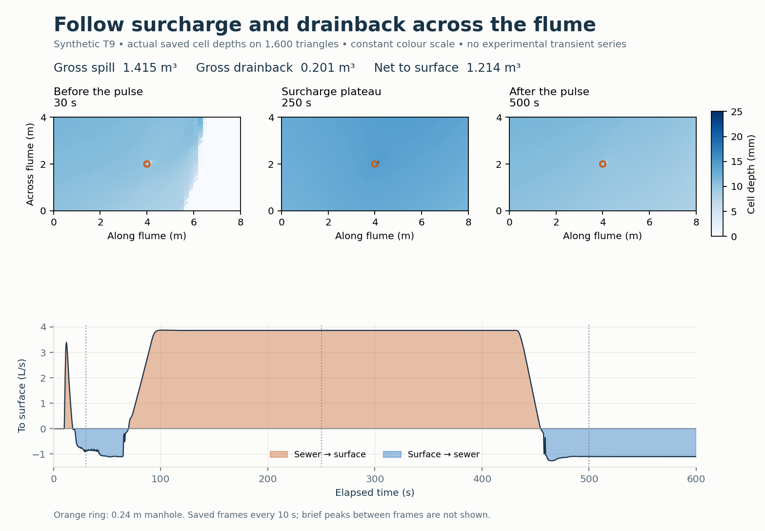
The maps use a fixed 0–25 mm colour scale; the orange ring marks the manhole. The vertical markers identify their times on the hydrograph. Surface inflow continues throughout the run, so the map includes both inflow and surcharge water. In the viewer, use Play, Restart, the speed selector and the frame slider to inspect the saved states. Gross spill and gross drainback update alongside the displayed time. The depth fields are saved every 10 s and are not interpolated; their maximum is 20.909 mm, while the all-step maximum is 24.803 mm. The native hydrograph retains the routing-step samples. These figures are calculated from saved results, rather than screenshots of the application.

Compare with the steady measurements

Run each steady input. Use the automated benchmark CSV for late-window exchange: it exports the 240-300 s mean and compares it with 180-240 s. The end-of-run report totals divided by 300 s give a whole-run average, not the last-minute rate. Only compare a rate as steady when those windows agree acceptably and both domain ledgers are acceptable. The full review includes all rows; the four supplied steady inputs are only the first row of each scenario.

Scenario	Measurement in the supplied seed (L/s)	Meaning
S1	0.69	Free-weir drainage, no sewer inflow
S2	0.24	Submerged-weir drainage near the crest
S3	1.73	Surcharge onto a wet floodplain
S4	1.74	Surcharge with no incoming surface flow

Do not treat a successful run or recovered regression slope as an experimental pass. Only 8 of 36 physical-shaft rates at the review's 0.5 s step lie in the illustrative measurement-variation-plus-2% comparison band, and some rates are not temporally converged. The paper's Table 3 slopes belong to fits with nonzero intercepts. Its wet outward orifice value is not an independently calibrated inward-orifice coefficient.

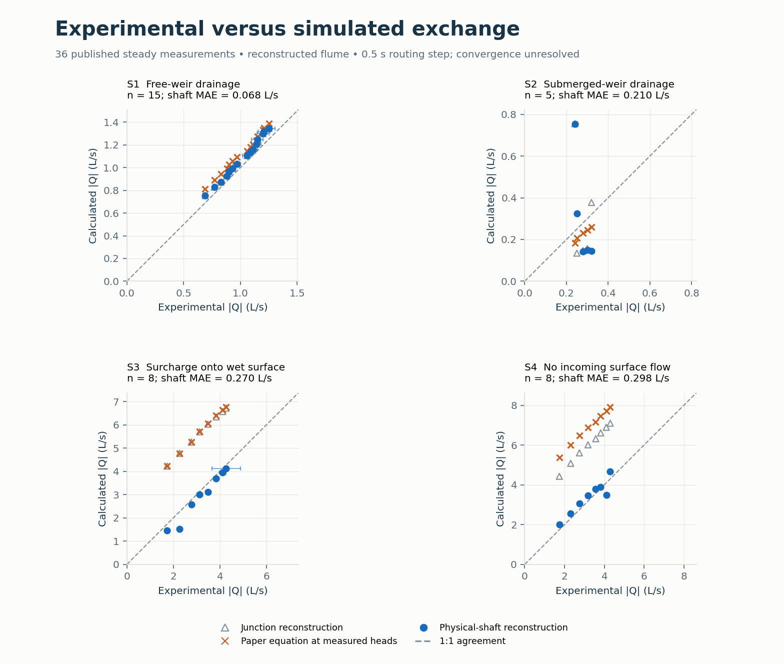
Experimental versus simulated steady exchange for all 36 Table 2 measurements

Blue points show the physical-shaft model, open triangles the original junction model, and orange crosses the bare paper equations evaluated at measured heads. The dashed line is 1:1 agreement. Horizontal error bars show the paper's measurement variation \(\xi_f\). Both axes within each panel use the same scale; the scale changes between regimes. MAE describes the physical-shaft absolute residual in L/s. All full-engine points here use the review's 0.5 s step and remain subject to convergence checks.

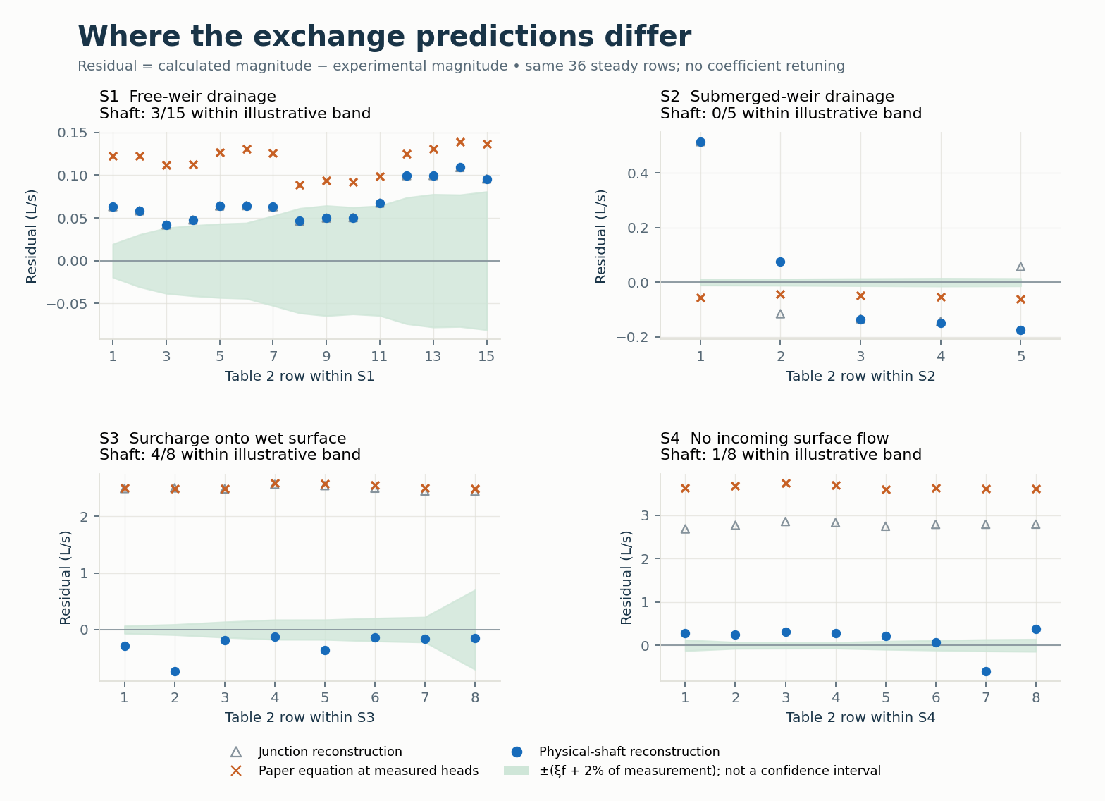
Exchange residuals by experimental row; shaded comparison band is not a confidence interval

Residuals are calculated minus measured discharge magnitudes. The green band is \(\pm(\xi_f+0.02Q_e)\), an illustrative comparison criterion. Row numbers restart within each regime. The points and band retain the disagreements that a successful run alone cannot reveal.

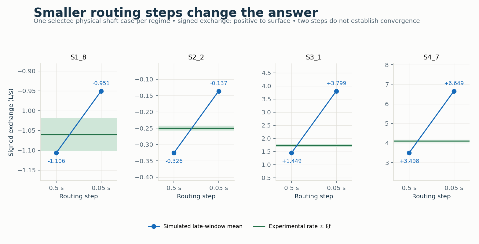
Selected experimental rates compared with physical-shaft results at two routing steps

Green lines/bands show the signed experimental rate and \(\xi_f\). The blue points show how reducing the routing step changes the late-window mean in one selected case per regime. Positive is sewer to surface. These four reruns do not establish convergence of the full matrix.

Fixed-time smoothing and convergence — 22 October follow-up

The figures above preserve the 21 October review. The follow-up changes the numerical smoothing schedule, with physical coefficients and geometry held fixed. In a copy of a steady input, open Simulation Options → 2D Surface Routing → Hydraulics. Under Explicit marcher set Momentum θ to 0.8 and Smoothing reference interval to 1 s. The engine key is THETA_REFERENCE_STEP. Zero means the original per-step smoothing; older engines disable the new control.

Keep the 1 s reference fixed in three copies with routing steps 0.0125, 0.00625 and 0.003125 s. To match the study, use maximum 1D trials 80, head tolerance 0.00001 m, variable step 0 and lengthening step 0. These are numerical controls; the reference interval was not fitted to measurements. Compare mean exchange over 240–300 s, the preceding minute, heads and separate 1D/2D continuity. The supplied steady examples are the first row of each regime; the download includes every Table 2 row and identifies each case.

All 36 cases meet the 1% final timestep-change criterion (maximum 0.516%) and the separate 2% drift/ordinary 1D continuity checks. 0/36 meet the illustrative experimental comparison band. This improves numerical consistency; experimental qualification remains incomplete.

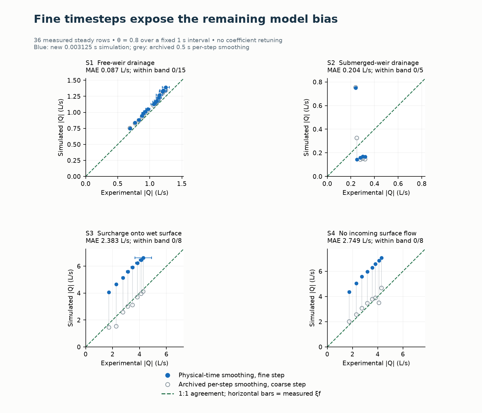
Fine-step physical-time model results compared with all 36 measured rates and the archived coarse-step results

Blue filled circles are the new simulated rates at 0.003125 s. Gray open circles are the older 0.5 s per-step results. The green dashed line shows 1:1 agreement and horizontal bars the measured variation. The new points expose the remaining model bias; they do not establish experimental validation.

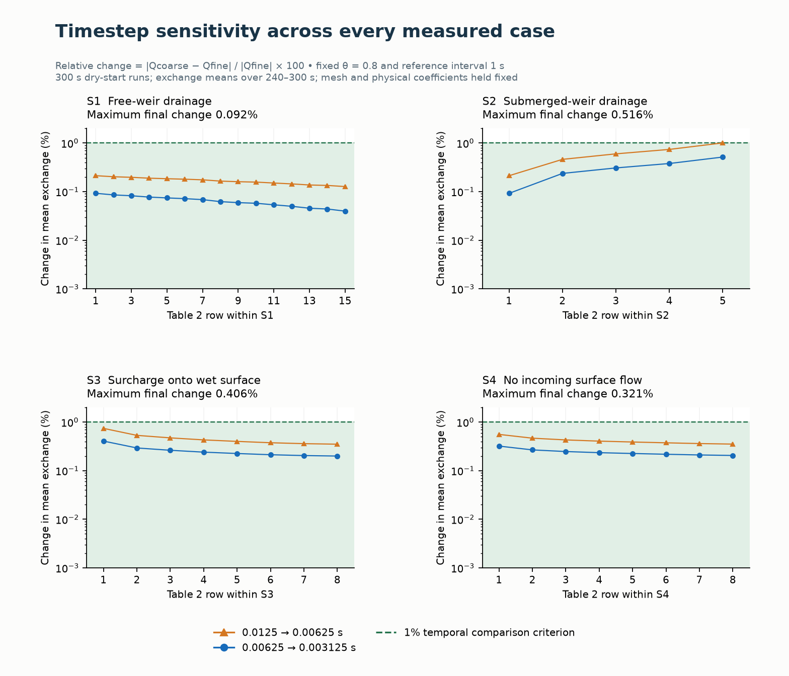
Relative exchange changes across two timestep halvings with the same smoothing interval

Orange triangles show 0.0125 → 0.00625 s and blue circles 0.00625 → 0.003125 s. Green shading is below the 1% comparison criterion; the ordinate is logarithmic. The single-cell delivery and spatial-convergence limitations remain.

Download the follow-up report and reusable figures, 36-case comparison table, and plotted data, heads and separate volume ledgers. The original transient viewer retains its original settings; no measured transient validation is added by this steady refinement study. Positive reference intervals require compatible engine support and surface GPU plugins at ABI 9.

Variations

Run copies with 0.1 s and 0.05 s routing steps. Compare late-window rates, head, gross transfer and continuity. Smaller drift is useful, but a change of mean rate between steps means time convergence remains open.
Compare lower/expected/upper coefficient presets. This is a parameter sensitivity; the resulting envelope is not a confidence interval.
Compare CELL and STENCIL_WET_MEAN head sampling. Record the selected cell positions and heads; these options do not reproduce the paper's exact pressure transducer or complete circular-opening average.
Refine the mesh in a copy while preserving the physical structure and its only intended coupling. Compare the sampling and delivery footprint. The existing fine-mesh anti-choking test is not a mesh-convergence result.

What remains unvalidated

The measured transient sewer-head and exchange series have not been replayed. Table 1's ratios/durations do not determine those series. The synthetic demonstration cannot reproduce the paper's observed suction oscillation or establish transient experimental accuracy. The hydraulic reference insert and illustrated review state the regularisation, single-cell delivery and time-step limitations that require further work.

Reference: Rubinato et al. (2017), Journal of Hydrology 552, 421-432.

T4 — Spill and Drainback Between a Pipe Network and a 2D Plaza — synthetic plaza spill and drainback
14 — Hydraulics: Nodes, Links, Cross-Sections, Streets, Inlets and Controls — node coupling properties
18 — Simulation Options — exchange law and head sampling
21 — Results Layers, Result Styling and Animation — 1D/2D result association