 |
OpenSWMM Engine
6.0.0-alpha.4
Data-oriented, plugin-extensible SWMM Engine (6.0.0-alpha.4)
|
|
OpenSWMM Engine
6.0.0-alpha.4
Data-oriented, plugin-extensible SWMM Engine (6.0.0-alpha.4)
|
A design storm arrives at a model with no history. A continuous simulation does not: what a storm produces depends on how wet the ground already is, how cold it has been, and what the last storm left behind.
Three additions to the hydrology serve that, and this chapter runs the one whose effect is largest and least obvious — a physics-based recovery for rainfall-derived inflow and infiltration, where the same storm produces a different answer in January than in June, in the same model, with no seasonal parameter table.
Deck: docs/figures/decks/hydrology_additions/rdii_decay.inp
One sanitary sewer node fed by an RTK unit hydrograph group over a 30-day January. Two identical six-hour storms fall nineteen days apart. The air temperature series warms through the month, and the chapter's second run lowers it below freezing.
The RTK group is the classic one — three response terms, one line each:
What is new is a decay row per response:
k_dep depletes the abstraction store per inch of rainfall; k_0 and k_T are the base and thermal recovery rates; θ_rec is the temperature sensitivity; and below T_freeze recovery stops entirely. The recovery needs a temperature source:
Two unit traps, both real. T_ref and T_freeze are in degrees Celsius whatever the project's units are. This is a US deck, so its temperature series is Fahrenheit and the engine converts before evaluating the recovery — a T_freeze of 0 means freezing, not −18 °C. And when a decay row is present the [HYDROGRAPHS] linear recovery rate is ignored for that response, while Dmax and D0 still apply, because they describe the reservoir rather than its dynamics.
The deck also selects the modified Green-Ampt variant:
which is the infiltration choice this chapter's kind of model wants. The original resets the cumulative infiltration whenever the inter-event timer expires; the modified variant does not, so a long drizzle below the saturated conductivity counts toward saturating the soil instead of being forgotten (Hydrology 4, §4.4.5).
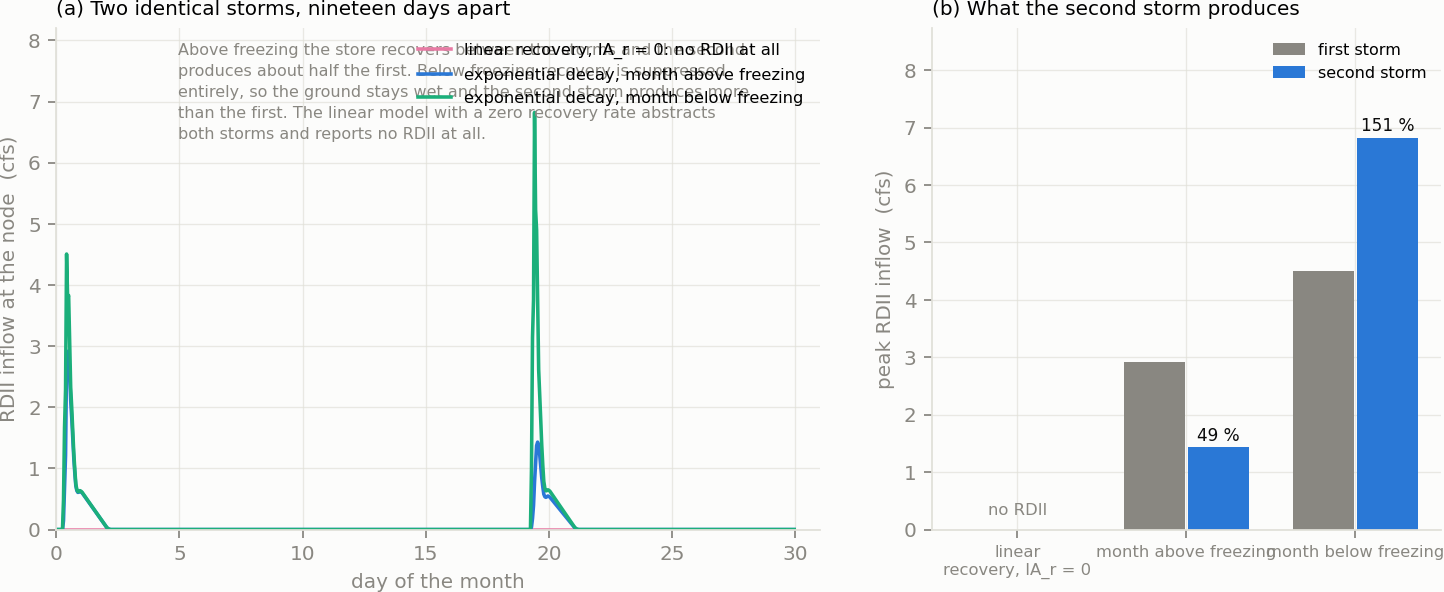
Figure 11-1 Two identical storms through one RTK group, with and without a physics-based recovery
| Run | First storm peak | Second storm peak | Second as a share |
|---|---|---|---|
Linear recovery, Drec = 0 | — | — | no RDII at all |
| Exponential decay, month above freezing | 2.921 cfs | 1.430 cfs | 49 % |
| Exponential decay, month below freezing | 4.505 cfs | 6.821 cfs | 151 % |
Table 11-1 The same two storms under three configurations
The second storm is not the first storm. Above freezing, the abstraction store recovers over the nineteen dry days but not completely, and the second storm produces 49 % of the first peak and 64 % of its volume. An RTK group with a fully recovered linear abstraction would have produced the same answer twice.
Below freezing, the ground stops recovering and the order reverses. With the month held under 0 °C, recovery is suppressed outright, so the store stays depleted, the first storm produces more than it did in the warm month, and the second produces more than the first — 151 %. That is the seasonal behaviour the section exists for, and it is the sign a lumped seasonal multiplier usually gets wrong.
The third run is a trap worth knowing. With the decay section removed this deck reports no RDII at all. Its [HYDROGRAPHS] rows carry an 8 in maximum abstraction with a recovery rate of zero, so the linear model abstracts both storms entirely and the run is silent about it: the continuity block simply shows 0.000 for RDII inflow. A model that reports no RDII is not necessarily a model with none.
Scale factors, at two levels. A gage carries a snow catch factor and a scale factor, and a subcatchment carries its own; the gage factor is applied inside the gage's reading, and the subcatchment factor after the conversion to internal units (Hydrology 2, §2.1.6). The rain-snow split sits between them, and the catch factor applies on the snow branch only. For a long run driven by one regional gage, that pair is how a subcatchment gets its own exposure without a second series.
Forcing from outside the deck. A continuous simulation often needs inputs a deck cannot hold — a downscaled climate series, an evaporation estimate computed from other variables, a live feed. Those are prescribed at runtime:
Prescribed values enter after the rain-snow split and are not scaled by either factor, which is what lets them drive a deck whose gages stay in place. Chapter 12 and the forcing guide carry the full set.
 1.13.2