 |
OpenSWMM Engine
6.0.0-alpha.4
Data-oriented, plugin-extensible SWMM Engine (6.0.0-alpha.4)
|
|
OpenSWMM Engine
6.0.0-alpha.4
Data-oriented, plugin-extensible SWMM Engine (6.0.0-alpha.4)
|
Chapters 2 through 7 describe hydrology on a lumped land surface: each subcatchment receives one rainfall intensity from one gage, converts it to runoff through one infiltration model and one nonlinear reservoir, and delivers the result to one outlet. Everything that happens between the rain and the outlet is integrated over the subcatchment's area before the conveyance system sees it.
The two-dimensional overland-flow mesh of Hydraulics Chapter 9 offers a second, distributed representation of the same surface. Rain can be applied to every cell of the mesh, each cell can infiltrate through its own soil parameters, and each cell evaporates from its own water. Runoff is then not a subcatchment quantity at all: it is the depth field the shallow-water solver routes over the terrain, and it enters the network wherever the terrain and the coupling points put it. This chapter documents those three cell-level processes — rainfall, infiltration and evaporation — and how they are accounted for. The mesh's own subsurface, which can receive the infiltrated water, is Chapter 9.
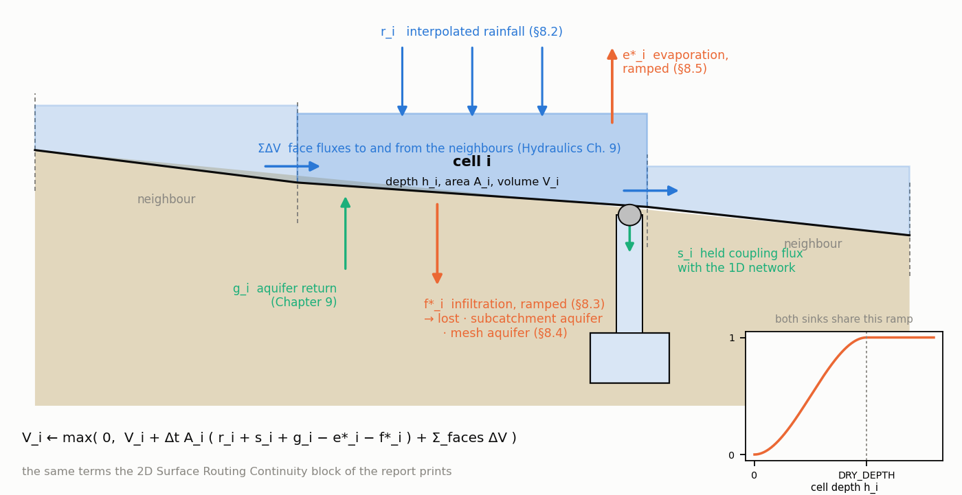
Figure 8-1 The water balance of one mesh cell: rainfall, evaporation, infiltration, network exchange and the lateral face fluxes
When rain on the mesh replaces subcatchment runoff. Water reaches the mesh by four routes — rainfall on the cells, spill from surcharged nodes, outfall discharge and boundary inflow — and only the first is hydrology in the sense of this manual. It is on by default: a project with a mesh and rain gages rains on the mesh unless told not to. Three configurations are intended. In rain-on-grid the mesh covers the catchment with no subcatchments over it; every cell receives rain, infiltrates (§8.3) and drains to the network across the terrain, and the subcatchment machinery of Chapters 3 and 4 is not involved. In a network-fed surface the subcatchments convert the storm as before and the mesh only routes what the network cannot hold; [2D_OPTIONS] RAINFALL_MODE NONE keeps rain off it. A hybrid has subcatchments over part of the terrain and rain on the mesh elsewhere.
The double-counting rule. Where a subcatchment polygon and rained-on mesh cells cover the same ground, the same storm is delivered twice — as runoff at the outlet node and as depth on the cells — and the outfall volume is wrong by exactly the overlap. The engine does not detect this for rainfall: RAINFALL_MODE is the modeller's statement of which representation owns the surface, and NONE is a modelling decision, not an optimisation. The one check is in the surface-quality resolver, which warns when a [2D_COVERAGES] cell lies inside a subcatchment carrying its own [COVERAGES]. A related consequence: because the mesh reads every gage, a gage no subcatchment names is now used and its state machine advances, where the legacy rule held its first record for the whole run.
[2D_OPTIONS] RAINFALL_MODE selects how the project's gages map onto the cells:
| Mode | Cell value |
|---|---|
NATURAL_NEIGHBOUR (default) | Spatial interpolation of the located gages onto each cell centroid: Laplace natural-neighbour weights inside the convex hull of the gages, inverse-distance weights outside it |
NEAREST_NEIGHBOUR (alias NEAREST_NEIGHBOR) | The reading of the single closest located gage, inside or outside the hull; an exact distance tie goes to the gage listed first. A dry closest gage keeps the cell dry |
SYSTEM | One uniform value, the arithmetic mean of every gage's current intensity |
NONE | No rain on the mesh |
A gage is located when it has a [SYMBOLS] coordinate; a coordinate of exactly (0, 0) marks it un-located and excludes it. Only the first of two coincident gages is kept, since the triangulation would otherwise degenerate. With no located gage at all, NATURAL_NEIGHBOUR and NEAREST_NEIGHBOUR fall back to the SYSTEM mean. Initialisation reports, as warnings, the number of un-located, non-finite and duplicate gages it skipped, the SYSTEM fallback, and the number of cells that received inverse-distance weights. The environment variable OPENSWMM_2D_RAINFALL_MODE (natural, nearest, system, none) overrides the deck key at initialisation.
Gage positions do not change during a run, so the interpolation is split into a one-time construction of per-cell weights and a per-step sparse weighted sum. For cell \(i\) with weights \(w_{ig}\) over the located gages \(g\), the cell rainfall is
\[ r_i = \sum_{g} w_{ig}\, R_g, \qquad \sum_{g} w_{ig} = 1 \]
(8-1)
where \(R_g\) is gage \(g\)'s current intensity converted to m/s. Because the conversion is linear, converting then interpolating equals interpolating then converting.
Inside the hull — Laplace (non-Sibsonian) natural-neighbour weights. The Delaunay triangulation of the gage sites is built by a self-contained Bowyer–Watson insertion (gage counts are small, typically under thirty, so no geometry library is involved). A cell centroid \(p\) is inside the hull when it lies in some Delaunay triangle. Inserting \(p\) as a new site carves a cavity — the triangles whose circumcircles contain \(p\) — and fans it with triangles \((p, u, v)\) over the cavity's boundary edges. The Voronoi facet between \(p\) and a boundary site \(s\) runs between the circumcentres of the two fan triangles incident to \(s\), and the Laplace weight is that facet's length divided by the distance to the site:
\[w_{ps} = \frac{\ell_{ps}}{\lvert p - x_s \rvert}, \qquad \ell_{ps} = \bigl\lvert c(p, s_{\mathrm{prev}}, s) - c(p, s, s_{\mathrm{next}}) \bigr\rvert \]
(8-2)
with \(c(\cdot)\) the circumcentre and the weights normalised to sum to one. Laplace weights reproduce a linear field exactly inside the hull and need no polygon-area integration, which distinguishes them from Sibson's weights. A centroid coincident with a gage takes that gage alone.
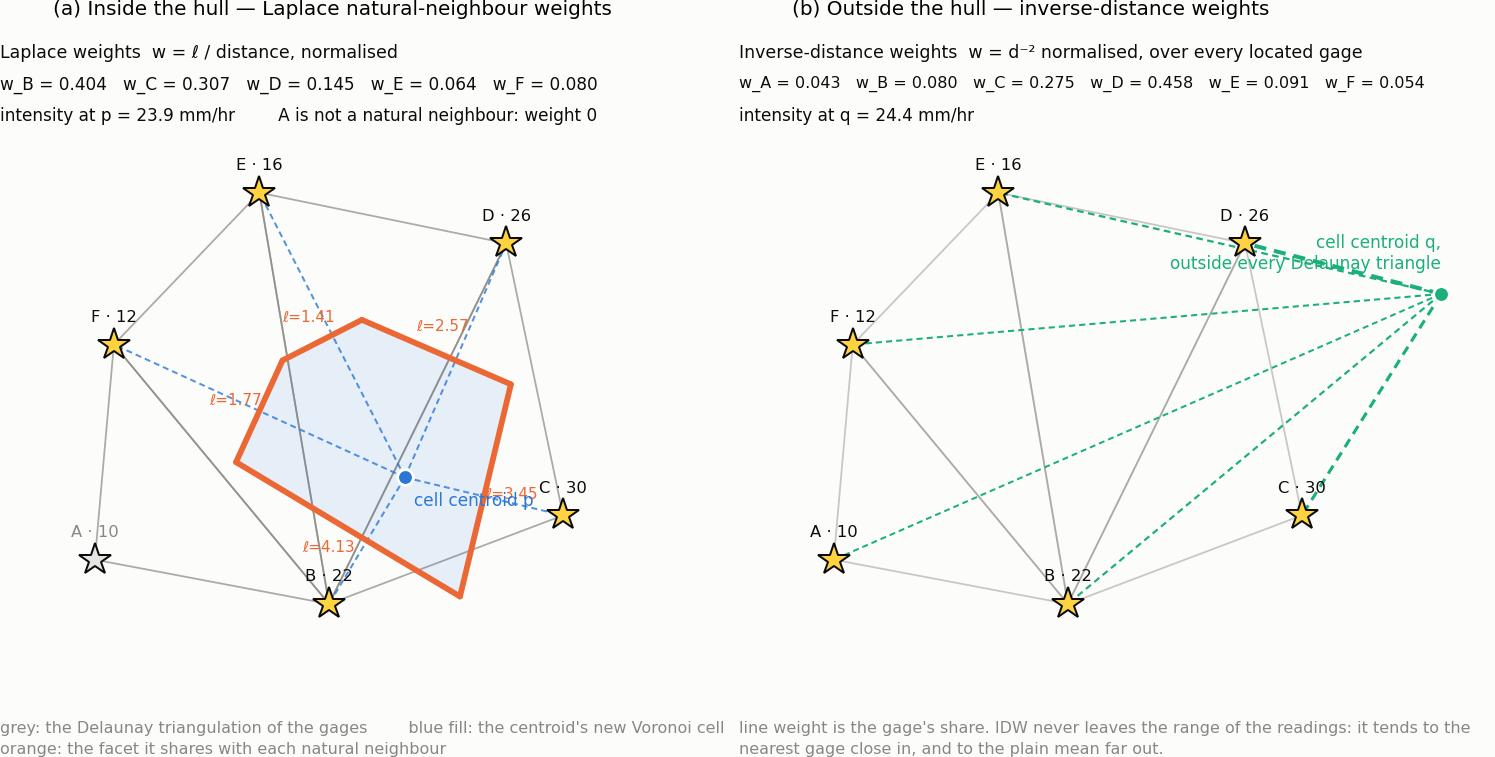
Figure 8-2 Natural-neighbour rainfall weights inside the gage hull, and inverse-distance weighting outside it
Outside the hull — inverse-distance weights. A centroid outside every Delaunay triangle, or one whose fan construction degenerates (a collinear fan triangle), takes power-2 inverse-distance weights over all located gages:
\[ w_{pg} = \frac{1 / d_{pg}^{2}}{\sum_{g'} 1 / d_{pg'}^{2}}, \qquad d_{pg} = \lvert p - x_g \rvert \]
(8-3)
IDW never leaves the range of the gage readings, tends to the nearest gage as the cell approaches it, and to the plain mean far from every gage.
Degenerate site sets. One located gage gives that gage everywhere; two, or three or more all collinear (an empty triangulation), give IDW everywhere; three or more non-collinear gages give Laplace inside the hull and IDW outside. Gage coordinates are in project map units and the centroids in SI metres, so the same feet-to-metres factor the mesh received is applied to the gage coordinates before triangulation.
Rainfall on the cells is refreshed with the other forcings on the co-advance cadence: at the first step, whenever a forcing prescription changes, and otherwise every 30 s of simulated time. Between refreshes each cell's intensity is held. Per-cell rainfall forcing through the API then overrides (OVERRIDE) or augments (ADD) the interpolated value.
Take three gages A, B and C at the corners of a triangle covering most of a mesh, reading 10, 20 and 30 mm/hr; the hull is that triangle.
[SYMBOLS] coordinate it would be excluded; the remaining pair is collinear, every cell becomes an IDW cell over A and B, and C's reading never reaches the mesh (it still drives any subcatchment naming it).SYSTEM every cell receives 20 mm/hr; under NONE, nothing.Infiltration on the mesh is a held rate, not a quantity evaluated inside the marcher. Every INFIL_STEP seconds the hydrology kernels of Chapter 4 are advanced once for every cell that carries a model, and the resulting capacity is published as a per-cell rate \(f_i\) (m/s) that the shallow-water substeps consume unchanged until the next evaluation. Evaluating the kernels per substep would be a different model — the Chapter 4 kernels are written for the runoff step — and would drag infiltration into the local-time-stepping tiers.
The cadence resolves as [2D_OPTIONS] INFIL_STEP, else [2D_INFILTRATION_OPTIONS] INFIL_STEP (the older home of the same value), else the project's WET_STEP. At initialisation the kernels are advanced once so the very first substep infiltrates rather than running a whole cadence dry; thereafter they receive the true elapsed interval. Kernel state is advanced for every model-carrying cell, including cells the marcher has deactivated as dry: a cell that sat inactive through a dry spell must not present its full initial capacity when rain arrives — its Horton capacity should have recovered and its Green-Ampt upper zone drained, as a subcatchment's would.
The cell-level methods are the Chapter 4 kernels, called through the same functions the runoff module calls and therefore bit-for-bit the same arithmetic:
| Method token | Kernel | Positional parameters (project units) |
|---|---|---|
HORTON | horton_getInfil (§4.2) | f0, fmin, decay (1/hr), dry time (d), Fmax |
MODIFIED_HORTON | modHorton_getInfil (§4.3) | f0, fmin, decay (1/hr), dry time (d), Fmax |
GREEN_AMPT | grnampt_getInfil (§4.4) | suction S, Ks, IMD |
MODIFIED_GREEN_AMPT | grnampt_getInfil with the modified flag (§4.4.5) | suction S, Ks, IMD |
CURVE_NUMBER | curvenum_getInfil (§4.5) | CN, (unused), dry time (d) |
CONSTANT | constant_getInfil | rate |
Rates (f0, fmin, Ks, rate) are in in/hr or mm/hr and depths (S, Fmax) in inches or mm, matching what a user types in [INFILTRATION]; the *_init functions convert them exactly as the runoff module does. CONSTANT is stored as a degenerate Horton state with \(f_0 = f_{min}\) and no decay, which gives it the same unit conversion for free. The curve-number row keeps the legacy column layout, so its drying time is the third value and the second is ignored.
The kernels work in feet and ft/s for every project; the 2D solver is SI. All conversion happens at the call boundary: the cell's rainfall and depth go in as feet, and the returned rate is scaled by 0.3048 and floored at zero:
\[ f_i = \max\bigl(0,\; 0.3048\, f_{\mathrm{kernel}}(3.2808\, r_i,\; 3.2808\, h_i,\; \Delta t_{infil})\bigr) \]
(8-4)
A mesh cell has no run-on from a neighbouring subarea, so the ponded depth is passed to the curve-number kernel unchanged where the runoff module would fold inter-subarea run-on into it.
Parameters resolve once, at initialisation, in the order
\[\text{cell override} \;>\; \text{TAG row} \;>\; \text{`*' row} \;>\; \text{none} \]
from three sections: [2D_INFILTRATION_DEFAULTS] (TAG METHOD [P1..P5] [DEST], where the tag * is the mesh-wide fallback and may appear anywhere), [2D_INFILTRATION] (CELL METHOD [P1..P5] [DEST], cells 1-based in the file) and [2D_INFILTRATION_OPTIONS] (INFIL_STEP). A TAG or CELL row whose method is NONE deliberately clears the * default for its cells. A - in a parameter column leaves that parameter unset. The solver never consults tags; the provenance of each cell's parameters is retained only so the writer can re-emit a compact file rather than one row per cell.
Three [2D_OPTIONS] keys sit above the sections. INFILTRATION YES|NO|AUTO is the process enable: AUTO (unset) runs infiltration when any row resolved, NO keeps the rows but deactivates them for the run (with a warning), and YES with nothing resolved warns that no cell infiltrates. INFIL_DEFAULT_METHOD names the method of the * row and must agree with it, since the parameters belong to the row: a mismatch is an error, a missing row a warning, and NONE drops the * row. INFIL_DESTINATION is §8.4. Validation refuses negative Horton rates, negative Ks, an IMD outside 0..1, a curve number outside 1..100, a negative constant rate, and a cell index beyond the mesh.
The marcher consumes the held rate through a depth-limited sink. For a cell of depth \(h_i\) and the solver's DRY_DEPTH \(h_d\),
\[f^{\ast}_i = \begin{cases} 0 & h_i \le 0 \\ f_i\, t^{2}(3 - 2t), \quad t = h_i / h_d & 0 < h_i < h_d \\ f_i & h_i \ge h_d \end{cases} \]
(8-5)
The cubic Hermite ramp is the same one the evaporation sink uses, so both sinks shut off together as a cell dries. The cell's volume update in every tier is then
\[V_i \leftarrow \max\Bigl(0,\; V_i + \Delta t\, A_i\,\bigl(r_i + s_i + g_i - e^{\ast}_i - f^{\ast}_i\bigr) + \sum_{\text{faces}} \Delta V\Bigr) \]
(8-6)
with \(s_i\) the held coupling flux, \(g_i\) the aquifer's return (Chapter 9, zero without an aquifer) and \(e^{\ast}_i\) the ramped evaporation. The plan states the sink order as rainfall, then evaporation, then infiltration "against the remaining depth"; in the code both sinks are evaluated from the same start-of-substep depth and summed, and the floor at zero in (8-6) is what keeps a cell non-negative. The two agree in effect, since both ramps vanish together, and a project with no infiltration rows is bitwise unchanged. The applied depth \(f^{\ast}_i \Delta t\) is accumulated per cell as it is removed, in active and lazy tiers alike and before any early exit (rain exactly cancelling the sink still infiltrated); that accumulator, not a re-derivation from the end-of-step depth, is what the ledger and the cumulative output read.
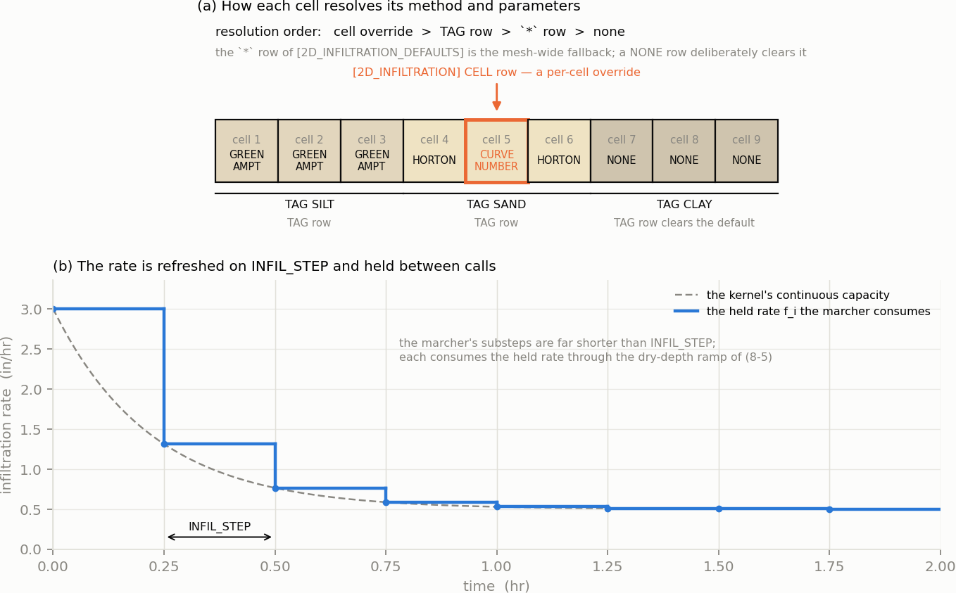
Figure 8-3 Per-cell infiltration: how a cell resolves its method and parameters, and the rate held across an infiltration step
Where infiltrated water goes is a per-row DEST column, defaulted for rows that do not spell one by [2D_OPTIONS] INFIL_DESTINATION:
| Destination | Meaning |
|---|---|
LOST (default) | Leaves the modelled system; booked as the 2D surface ledger's infiltration loss |
SUBCATCH_AQUIFER | Recharges the legacy per-subcatchment aquifer of Chapter 5 that contains the cell |
AQUIFER_2D | Recharges the two-zone mesh aquifer of Chapter 9 |
The writer emits DEST only for rows that spelled it, so a deck round-trips unchanged.
AQUIFER_2D is legal exactly when a [2D_AQUIFER] section resolved. Without one it is refused with a message naming the section to add, rather than read as LOST: silently draining a model the author believed was recharging is the worse failure.
SUBCATCH_AQUIFER resolves each routed cell to the subcatchment whose [Polygons] contain its centroid (ray-crossing test in map units); the first by index wins, an overlap is reported once, and cells outside every polygon stay LOST with a warning. The marcher does not deliver the recharge: the applied depth is accumulated per subcatchment on the once-per-routing-step ledger pass, and the runoff step drains the accumulator, converts it to a rate over the full subcatchment area and adds it to that subcatchment's infiltration rate before the groundwater solver runs. It is booked to the 1D groundwater ledger and to the 2D ledger's "to Aquifer (delivered)" row at the moment of delivery, so the two ledgers sum the same volumes; the applied but not yet drained remainder is the "in flight" row. Because a subcatchment's aquifer has one owner, the destination is refused alongside the registered org.hydrocouple.openswmm.integrated2d component or a [2D_AQUIFER].
The aquifer owns infiltration. With a [2D_AQUIFER] present, every infiltrating cell's water is booked to the cell's aquifer column — in the active tier and in the lazy tier alike — whatever its DEST token says. LOST then reads as AQUIFER_2D. That is what a user means by putting an aquifer under the mesh, and it keeps the water to one owner. The 2D surface ledger still prints the volume as "Infiltration Loss", since it left the surface; the same volume appears as "Infiltration Inflow" in the aquifer's own block (Chapter 9 §9.10).
[2D_OPTIONS] EVAPORATION NO|YES|CLIMATE sets the base rate every cell evaporates at:
| Value | Base rate on an unforced cell |
|---|---|
YES (default) | Zero. Only per-cell forcing through the API (swmm_2d_force_evap*) evaporates — the behaviour before the key existed |
CLIMATE | The project's [EVAPORATION] rate, converted from the internal ft/s to m/s |
NO | Zero, and forcing is ignored |
This differs from the subcatchments and is worth stating plainly: a mesh with the default setting and no forcing does not evaporate, whatever [EVAPORATION] says; CLIMATE makes it follow the project's climate. Per-cell forcing replaces (OVERRIDE) or adds to (ADD) the base rate, on the same 30 s refresh cadence as rainfall.
The rate reaches the cell budget through the same depth-limited ramp as infiltration, (8-5) with \(e_i\) in place of \(f_i\), so a drying cell cannot evaporate more water than it has. Evaporation removes water and no solute: when species are transported on the mesh, both intensive rows are sunk at the cell's own mean so that concentrations rise, which is the up-concentration a drying pond should show.
The 2D domain keeps its own ledger in SI cubic metres, printed as a separate block after the flow-routing continuity when [REPORT] CONTINUITY is on. Its rows and how each is accumulated:
| Row | Accumulation |
|---|---|
| Initial Stored Volume | Surface volume at the start |
| Rainfall Inflow | \(\sum_i r_i A_i\, \Delta t\) per routing step, from the per-cell rate after forcing |
| 1D to 2D Spill Inflow, 2D to 1D Drain Outflow | Signed junction exchange, per node per batch |
| Outfall Inflow, Outfall Withdrawal | Signed outfall exchange |
| Boundary Inflow, Boundary Outflow | Non-wall boundary edges, outward-positive |
| Evaporation Loss | \(\sum_i e^{\ast}_i A_i\, \Delta t\) re-derived at the accepted end-of-step depth (exact while cells stay wetter than DRY_DEPTH, first-order through dry-out) |
| Infiltration Loss | The applied depth the marcher actually removed, summed as it was removed — not a re-derivation |
| to Aquifer (delivered), to Aquifer (in flight) | The SUBCATCH_AQUIFER share; printed only when non-zero |
| Final Stored Volume | Surface volume at the end |
The infiltration row is deliberately not re-derived from end-of-step state: re-deriving (8-5) at the accepted depth is first-order and under-books on exactly the cells that matter — a cell drying mid-step is sunk at the higher early-step rate, and the lazy tier integrates a stale depth across a whole sync interval. On the rain-on-grid gate that left 0.0117 m³ of a 3.775 m³ budget unaccounted.
The continuity error is
\[\varepsilon_{2D} = \frac{V_{in} - V_{out}}{V_{in}}, \qquad V_{in} = V_0 + R + S_{1D\to2D} + O_{in} + B_{in} + G_{in}, \quad V_{out} = V_1 + S_{2D\to1D} + O_{out} + B_{out} + E + F \]
(8-7)
with \(G_{in}\) the water a Chapter 9 aquifer returned to the surface (Dunne excess and top-layer rejection, less what is still waiting to be picked up). \(G_{in}\) enters the error but is not printed as a row of the block in this release.
Two REPORT_2D_VARIABLES groups, both in DEFAULT, carry the per-cell series:
| Group | Datasets | Content |
|---|---|---|
RAINFALL | Mesh2_face_rainfall, Mesh2_face_rain_cum | Per-cell rate after forcing (m/s) and cumulative depth |
INFILTRATION | Mesh2_face_infil_rate, Mesh2_face_infil_cum | The held rate (m/s) and the ledger-consistent applied cumulative depth (m) |
The cumulative series is SurfaceRouter2D::infilCumulative(), which drains the same applied-depth accumulator the ledger books, so \(\sum_i \mathrm{infil\_cum}_i A_i\) equals the Infiltration Loss row by construction; Infil2D::cumulative(), the integral of the unramped capacity the kernels offered, is a kernel-side diagnostic that exceeds the applied loss on drying cells. The C API's *_get_cum_bulk reports the former.
| Family | Alternative | Behaviour | Status |
|---|---|---|---|
| Rain mode | NATURAL_NEIGHBOUR | Laplace weights inside the gage hull, IDW outside; static weights | Implemented |
| Rain mode | NEAREST_NEIGHBOUR | Closest located gage, weight 1; first-listed gage wins a tie; static weights | Implemented |
| Rain mode | SYSTEM | Uniform mean of all gages; automatic fallback with no located gage | Implemented |
| Rain mode | NONE | No rain on the mesh; the subcatchments own the surface | Implemented |
| Infiltration | HORTON | Chapter 4 §4.2 kernel, per cell | Implemented |
| Infiltration | MODIFIED_HORTON | Chapter 4 §4.3 kernel, per cell | Implemented |
| Infiltration | GREEN_AMPT | Chapter 4 §4.4 kernel, per cell | Implemented |
| Infiltration | MODIFIED_GREEN_AMPT | Chapter 4 §4.4.5 variant, per cell | Implemented |
| Infiltration | CURVE_NUMBER | Chapter 4 §4.5 kernel, per cell, no run-on | Implemented |
| Infiltration | CONSTANT | Fixed rate, stored as a degenerate Horton state | Implemented |
| Destination | LOST | Exit from the modelled system | Implemented |
| Destination | SUBCATCH_AQUIFER | Delivered to the containing subcatchment's Chapter 5 aquifer at the runoff step | Implemented |
| Destination | AQUIFER_2D | Delivered to the Chapter 9 mesh aquifer; owns all infiltration when present | Implemented |
| Destination | Exfiltration (negative rate) from the ground to the mesh | Not a destination; the sink floors at zero. Return flow arrives through the Chapter 9 aquifer instead | Retired |
| Evaporation | YES | Forcing only | Implemented |
| Evaporation | CLIMATE | Project [EVAPORATION] rate on unforced cells | Implemented |
| Evaporation | NO | No sink, forcing ignored | Implemented |
| Concern | Where |
|---|---|
| Rainfall weights and application | src/engine/2d/mesh/RainfallInterpolator.hpp, .cpp — build() once from SurfaceRouter2D::initialize(), apply() from SurfaceRouter2D::updateRainfall() |
| Rain mode, process enables, evaporation mode | src/engine/2d/data/SolverOptions2D.hpp (RainfallMode, infiltration, infil_step, infil_default_method, infil_destination, evaporation); parsed in src/engine/2d/input/SectionHandlers2D.cpp |
| Per-cell infiltration state and kernels | src/engine/2d/infil/Infil2D.hpp, .cpp — resolve() at initialise, updateRates() on the cadence from SurfaceRouter2D::coAdvanceStep(); kernels in src/engine/hydrology/Infiltration.hpp |
| Section grammar | [2D_INFILTRATION_OPTIONS], [2D_INFILTRATION_DEFAULTS], [2D_INFILTRATION] in SectionHandlers2D.cpp; documented in [2D_INFILTRATION_OPTIONS], [2D_INFILTRATION_DEFAULTS] and [2D_INFILTRATION]; the [2D_OPTIONS] keys in [2D_OPTIONS], all in the input-file chapter |
| The sinks in the cell budget | src/engine/2d/solver/SurfaceFluxCalculator.hpp (evapSink, infilSink); consumed in src/engine/2d/solver/ExplicitInertialSolver.cpp (lazySourcesOnly, syncAndRebuild, fireCellsImpl) |
| Destination routing | SurfaceRouter2D::initialize() (validation, cell-to-subcatchment map), accumulateMassBalance() (per-subcatchment accumulation), src/engine/core/SWMMEngine.cpp runoff step (delivery); the marcher books to the Chapter 9 kernel directly |
| Ledger and report | SimulationContext::MassBalance2D; src/engine/plugins/DefaultReportPlugin.cpp (2D Surface Routing Continuity) |
| Results file | src/engine/2d/output/Default2DOutputPlugin.cpp (Mesh2_face_rainfall, _rain_cum, _infil_rate, _infil_cum); group masks in src/engine/2d/data/Report2DVars.hpp |
The design record is plans/TWO_ZONE_GROUNDWATER_EXPLICIT_LTS_PLAN_2026-08-15.md §5.5 (decisions D-I1 to D-I6). Two of its statements are superseded and this chapter follows the code: D-I4's "`LOST` is the only destination accepted" was amended when SUBCATCH_AQUIFER and AQUIFER_2D landed (§8.4), and the sequential sink ordering is realised as the summed, floored update (8-6).
 1.13.2