Problem

A pipe that is running part full begins to fill. A bore travels down it, the pipe pressurises behind the front, and whatever is at the downstream end — a manhole, a shaft, a surge tank — takes the water and oscillates.

A modeller has to decide how much of that to represent. The dynamic wave router carries one flow per conduit, so the bore is not a front it can place: the conduit fills as a whole. The finite-volume router discretises the conduit and the front is a cell boundary that moves. The question this chapter answers is what the difference is worth, measured against a laboratory pipe where the answer is known.

Deck

Deck: docs/figures/decks/rapid_fill/rapid_fill.inp

The rapid-filling experiment of Vasconcelos, Wright and Roe (2006): an acrylic pipe 14.33 m long and 94 mm in diameter, horizontal, initially at rest and 78 % full. A fill box feeds the upstream end and a 0.19 m surge tank closes the downstream one. At t = 0 an inflow of 3.1 L/s is admitted, and pressure at x = 9.9 m, velocity at the same station and the surge-tank level were all measured. The deck carries the paper's own numerics: 400 cells, Courant 0.95, Manning n = 0.012, acoustic celerity 25 m/s.

The two gauge stations are virtual junctions — sealed splices with no storage, transparent to the solution — so the deck also exercises the virtual-junction composition. docs/figures/decks/rapid_fill/provenance.md records where the deck and the three digitised measurement series came from.

Options that select the formulation

The deck as committed is the finite-volume router with its static slot:

[OPTIONS]
FLOW_ROUTING         FV
FV_CELL_LENGTH       0.036
FV_MIN_CELLS         4
FV_SLOT_CELERITY     25

The comparison runs change nothing else. The dynamic wave variants are

FLOW_ROUTING DYNWAVE

SURCHARGE_METHOD EXTRAN ; and, in the third run, SLOT

FV_CELL_LENGTH is the target cell length and FV_MIN_CELLS the floor; 0.036 m over 14.33 m is the paper's 400 cells. FV_SLOT_CELERITY is the pressurised wave speed the slot is sized for — the accuracy-cost trade of Hydraulics 8, §8.4.1, since the explicit step is bounded by \(\Delta x / (|v| + c)\).

Two warnings are expected and correct: INERTIAL_DAMPING and NORMAL_FLOW_LIMITED are dynamic wave keys, and the engine says so rather than ignoring them silently when the deck runs under FV.

Results

Figure 2-1

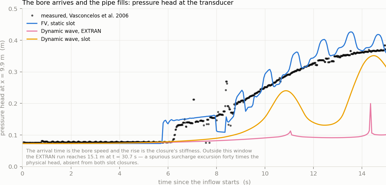
Figure 2-1 Pressure head at x = 9.9 m in the rapid-filling experiment, measured and under three routing choices

Figure 2-2

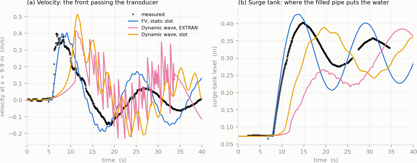
Figure 2-2 Velocity at the transducer and surge-tank level, measured and under the same three choices

	Front arrival at 9.9 m	Surge-tank first peak	Routing continuity error	Run time
Measured	6.26 s	0.403 m at 14.8 s	—	—
`FV`, static slot	5.80 s	0.427 m at 13.8 s	−0.000 %	17.3 s
`DYNWAVE`, slot	8.75 s	0.389 m at 19.6 s	1.147 %	0.1 s
`DYNWAVE`, EXTRAN	10.90 s	0.267 m at 19.5 s	5.655 %	0.2 s

Table 2-1 What each formulation reproduces, against the laboratory measurement

Arrival is the first time the head at the transducer passes 0.10 m; the surge-tank peak is the first maximum within 25 s. Every number comes from the runs this page's figures were drawn from.

The front. The finite-volume run puts the bore at the transducer half a second early and reproduces the whole rise; both dynamic wave runs are late by 2.5 s and 4.6 s. That is not a calibration difference. The dynamic wave router has no representation of a front inside a conduit, so the filling of the pipe is spread over the conduit's own storage rather than propagated; the arrival it reports is the arrival of a flow, not of a bore.

The oscillation. The surge tank is the honest test of what happens after filling, because its level integrates everything the pipe did. The finite-volume run peaks 0.024 m high and one second early; the dynamic wave runs peak five seconds late, and the EXTRAN run loses a third of the amplitude.

The velocity trace is where EXTRAN fails visibly. Panel (a) of Figure 2-2 shows it oscillating between ±0.2 m/s from about 13 s onward, at the reporting interval — numerical chatter, not a physical signal. The same run's flow-routing continuity error is 5.655 %, against −0.000 % for the finite-volume run. Outside the plotted window it reaches 15.1 m of head at the transducer, forty times the physical value.

What it costs. Seventeen seconds against a fifth of a second, on a deck of three conduits. The finite-volume router's step is bounded by the Courant condition on the shortest cell, and this deck is 400 cells of 36 mm; the ratio is the price of resolving the front. For a network model the ratio is smaller — cells are metres, not centimetres, and local time stepping (Hydraulics 8, §8.5.6) keeps the quiet parts of the network off the fine clock.

Which one to believe. Here, the finite-volume run, because a laboratory measurement says so. Away from a measurement, the discriminator is continuity: a routing error of 5.655 % on a three-pipe deck with no outfall losses is the solver reporting that it could not close its own books.

Where to go next

Chapter 3: a sub-atmospheric transient — the same pipeline with the centre raised and drained, where the static slot does not produce a wrong answer but no answer at all
Hydraulics 8 — the finite-volume scheme, its slot closure and its time stepping
Hydraulics 3 — the dynamic wave solver and its four surcharge methods
Section: [OPTIONS] — the grammar of every key named here
18 — Simulation Options — the same choices in the GUI