 |
OpenSWMM Engine
6.0.0-alpha.4
Data-oriented, plugin-extensible SWMM Engine (6.0.0-alpha.4)
|
|
OpenSWMM Engine
6.0.0-alpha.4
Data-oriented, plugin-extensible SWMM Engine (6.0.0-alpha.4)
|
This chapter describes how SWMM converts precipitation excess (rainfall and/or snowmelt less infiltration, evaporation, and initial abstraction) into surface runoff (overland flow). Because SWMM is a distributed model it allows a study area to be subdivided into any number of irregularly shaped subcatchment areas to best capture the effect that spatial variability in topography, drainage pathways, land cover, and soil characteristics have on runoff generation. Generation of runoff is therefore computed on a subcatchment by subcatchment basis.
SWMM uses a nonlinear reservoir model to estimate surface runoff produced by rainfall over a subcatchment. The model was first published by Chen and Shubinski (1971) and included in the original release of SWMM (Metcalf and Eddy et al., 1971a). Discussions of ancillary processes that serve as components of the runoff model, such as infiltration and snowmelt, are covered elsewhere in this manual.
SWMM conceptualizes a subcatchment as a rectangular surface that has a uniform slope S and a width W that drains to a single outlet channel as shown in Figure 3-1. Overland flow is generated by modeling the subcatchment as a nonlinear reservoir, as sketched in Figure 3-2.
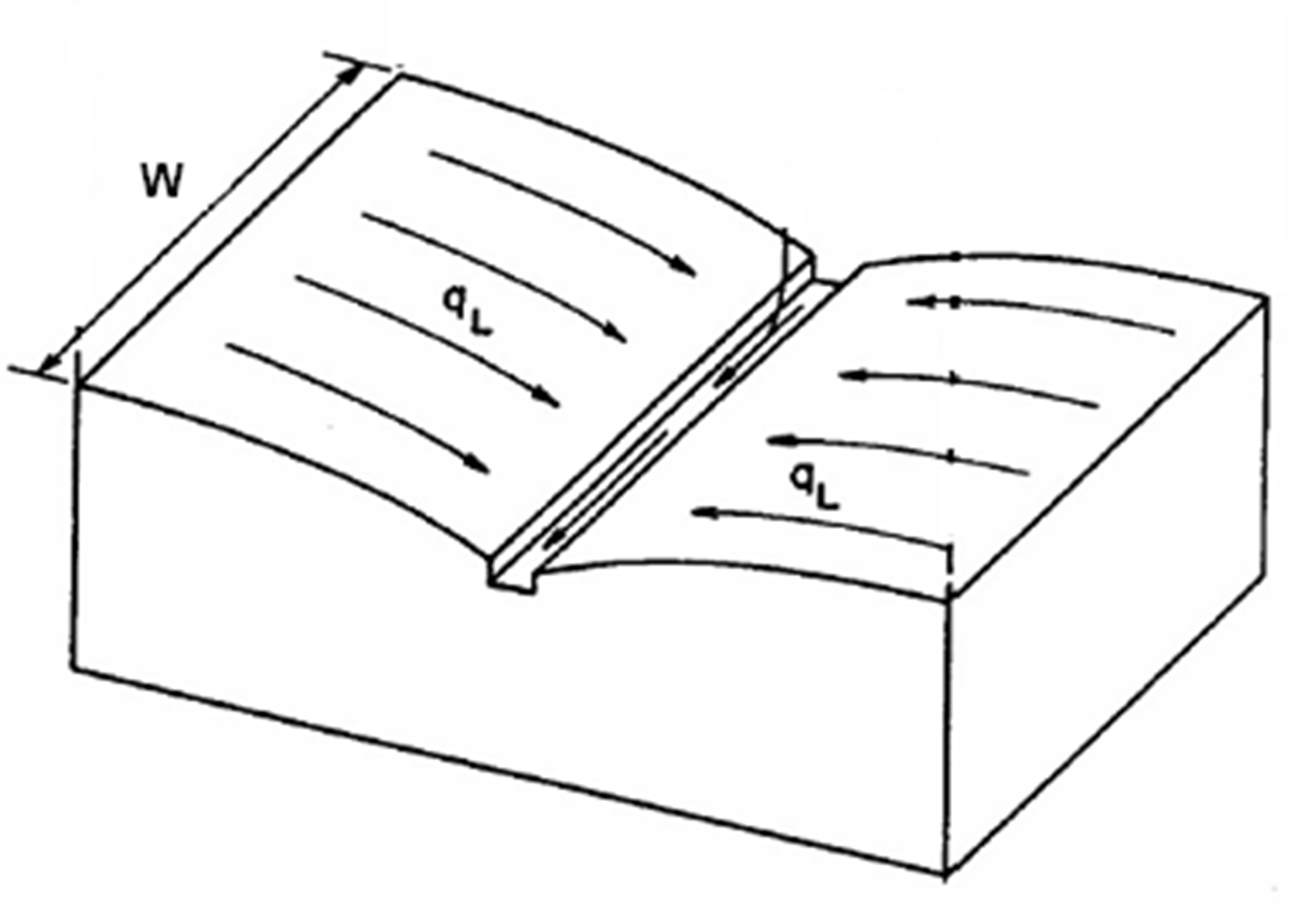
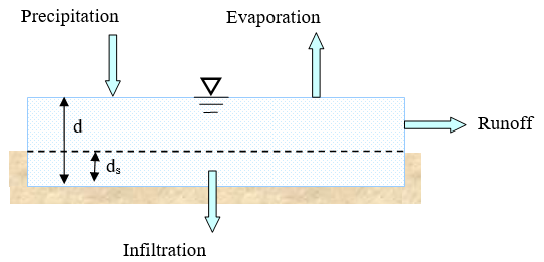
Figure 3-1 Idealized representation of a subcatchment.
Figure 3-2 Nonlinear reservoir model of a subcatchment.
In this representation, the subcatchment experiences inflow from precipitation (rainfall and snowmelt) and losses from evaporation and infiltration. The net excess ponds atop the subcatchment surface to a depth d. Ponded water above the depression storage depth d_s can become runoff outflow q. Depression storage accounts for initial rainfall abstractions such as surface ponding, interception by flat roofs and vegetation, and surface wetting.
From conservation of mass, the net change in depth d per unit of time t is simply the difference between inflow and outflow rates over the subcatchment:
\[\frac{\partial d}{\partial t} = i - e - f - q\]
(3-1)
where:
i = rate of rainfall + snowmelt (ft/s)
e = surface evaporation rate (ft/s)
f = infiltration rate (ft/s)
q = runoff rate (ft/s)
Note that the fluxes i, e, f, and q are expressed as flow rates per unit area (cfs/ft2 = ft/s).
Assuming that flow across the subcatchment's surface behaves as if it were uniform flow within a rectangular channel of width W (ft), height d - d_s, and slope S, the Manning equation can be used to express the runoff's volumetric flow rate Q (cfs) as:
\[Q = \frac{1.49}{n}S^{1/2}R_{x}^{2/3}A_{x}\]
(3-2)
Here n is a surface roughness coefficient, S the apparent or average slope of the subcatchment (ft/ft), A_x the area across the subcatchment's width through which the runoff flows (ft2), and R_x is the hydraulic radius associated with this area (ft). Referring to Figures 3-1 and 3-2, A_x is a rectangular area with width W and height d - d_s. Because W will always be much larger than d it follows that \(A_{x} = W(d - d_{s})\) and \(R_{x} = d - d_{s}\). Substituting these expressions into Equation 3-2 gives:
\[Q = \frac{1.49}{n}WS^{1/2}\left( d - d_{s} \right)^{5/3}\]
(3-3)
To obtain a runoff flow rate per unit of surface area, q, Equation 3-3 is divided by the surface area of the subcatchment, A (which should not be confused with the cross-section area A_x through which the runoff passes):
\[q = \frac{1.49WS^{1/2}}{A\ n}\left( d - d_{s} \right)^{5/3}\]
(3-4)
Substituting this equation into the original mass balance relation 3-1 results in:
\[\frac{\partial d}{\partial t} = i - e - f - \alpha\left( d - d_{s} \right)^{5/3}\]
(3-5)
where α is defined as:
\[\alpha = \frac{1.49WS^{1/2}}{A\ n}\]
(3-6)
Equation 3-5 is an ordinary nonlinear differential equation. For known values of i, e, f, d_s and α it can be solved numerically over each time step for ponded depth d. Once d is known, values of the runoff rate q can be found from Equation 3-4. Note that Equation 3-5 only applies when d is greater than d_s. When d ≤ d_s, runoff q is zero and the mass balance on d becomes simply:
\[\frac{\partial d}{\partial t} = i - e - f\]
(3-7)
The equation used to generate surface runoff was developed on the basis of an idealized rectangular subcatchment area with uniform properties. Urban areas usually contain a mix of land surface types which can conveniently be divided into two primary categories: pervious surfaces (e.g., lawns, fields, and forested areas) which allow rainfall to infiltrate into the soil and impervious surfaces (e.g., roofs, roads, and parking lots) over which no infiltration occurs. Therefore SWMM allows each subcatchment to have both a pervious and impervious subarea over which Equation 3-5 is solved. The user-supplied parameter Percent Imperviousness determines how much of the total subcatchment is devoted to each type of surface.
In addition, it is not uncommon for impervious surfaces to begin generating runoff almost immediately after a rainfall event occurs, well before its depression storage depth fills up. To model this behavior, SWMM allows the impervious area of a subcatchment to be further divided into two subareas: one with depression storage and one without. The input parameter % Zero-Imperv determines what fraction of a subcatchment's impervious area has no depression storage. Thus overall, a subcatchment can contain three types of subareas as shown in Figure 3-3. Note that under these definitions all impervious area is directly connected to the subcatchment's outlet point (typically a drainage pipe or channel). How to model indirectly connected areas, such as roof drains that discharge to pervious lawn areas, is discussed in section 3.6 below.
Figure 3-3 Types of subareas within a subcatchment.
Conceptually, these three sub-areas are incorporated into the idealized subcatchment as shown in Figure 3-4. Of course in reality the areas will not align in this fashion nor will they necessarily be compact and connected. The arrangement used here is merely a modeling convenience. Symbols A1, A2, and A3 refer to the pervious subarea and two types of impervious subareas (with and without depression storage), respectively, and they discharge their runoff independently of one another to the same outlet location.
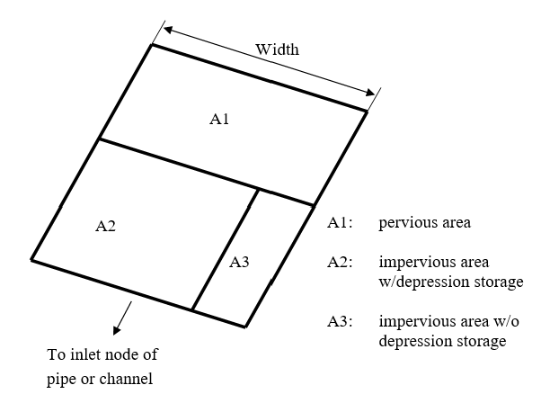
Figure 3-4 Idealized subcatchment partitioning for overland flow.
With this refinement the governing differential equation 3-5 for subcatchment runoff is solved individually for each subarea. Thus a separate accounting of the ponded depth d over each subarea is maintained. At the end of each time step, the runoff flows from each subarea are combined together to determine a total runoff flow for the entire subcatchment. The following conventions apply when solving the runoff equation for each subarea individually:
The applicable α-terms to be used in Equation 3-5 for each subarea are:
\[\alpha_{P} = \frac{1.49WS^{1/2}}{A_{1}n_{P}}\]
for the pervious subarea A1 (3-8)
\[\alpha_{I} = \frac{1.49WS^{1/2}}{\left( A_{2} + A_{3} \right)n_{I}}\]
for both impervious subareas A2 and A3 (3-9)
where n_P is the roughness for the pervious area, n_I is the roughness for both impervious areas, and A_i is the surface area (ft2) associated with sub-area i.
The reason that the same α applies to both impervious subareas even though their areas are different arises from how the W/A term is evaluated for the idealized arrangement shown in Figure 3-4. For area A2, W*₂ = *A*₂*W / (A*₂ + *A*₃) so that *W*₂ / *A*₂ = *W / (A*₂ + *A*₃). For A3, *W*₃ = *A*₃*W / (A*₂ + *A*₃) which results in *W*₃ / *A*₃ = *W / (A*₂ + *A*₃). Thus both types of impervious areas use the same factor *W / (*A*₂ + *A*₃).
The detailed computational scheme for computing the runoff generated from each subcatchment within a study area over a single time step of a simulation is presented below.
Computational Scheme for Runoff
\[Q = \sum_{j=1}^{3} q_j A_j\]
where q_j is the runoff per unit area in subarea j found in step 3 and A_j is the area of subarea j.The solution of Equation 3-5 at step 3.e of this process proceeds as follows:
a. If ponded depth is currently below the depression storage depth (d < d_s) and the rainfall excess is positive then determine the time step Δ*t_x* during which the depth will exceed d_s: Δ*t_x* = Δ*t* - (d_s - d)/*i_x* and set d = d_s. Otherwise set Δ*t_x* = Δ*t*.
b. Use a standard fifth-order Runge-Kutta integration routine with adaptive step size control (Press et al., 1992) to solve the equivalent of Equation 3-5,
\[\frac{\partial d}{\partial t} = i_x - \alpha d_x^{5/3}\]
for d over the time step Δ*t_x*. Here d_x = d - d_s for d > d_s and is 0 otherwise while α is α_P (Equation 3-8) if the subarea is pervious or is α_I (Equation 3-9) if the subarea is impervious.
c. Compute the runoff per unit area q at the end of the time step: q = αd_x5/3 where α and d_x are defined as above.
Recall that the depression storage d_s can have different user-supplied values for subareas A1 (pervious) and A2 (impervious) while it is zero by definition for subarea A3. Also note that initially at time zero the ponded depth d on each subarea of each subcatchment is zero.
SWMM allows the user to specify two different time steps that will be used when evaluating surface runoff during a simulation: a "wet" step and a "dry" step. The wet time step is used when there is precipitation or overland flow on any subcatchment within the study area. The longer dry time step applies when there is both no precipitation input and all depression storage remains unfilled.
Typically the wet time step will be an integer fraction of the rainfall interval. Five-minute rainfall might have wet time steps of 1, 2.5 or 5.0 min, for example. If the wet time step is not an integer fraction of or is larger than the rainfall interval, SWMM will automatically reduce the time step so that the rainfall intensity remains constant over the adjusted time step. A smaller wet time step would be desirable when the subcatchment is small and the time of concentration is a fraction of the rainfall interval. When using 1-hour rainfall, wet time steps of 10 min, 15 min or longer can be used by the model, unless subcatchments are very small. The key concept is that the wet step should be less than or equal to the response time of a subcatchment. Time of concentration, t~c~, is one measure of response time (Eagleson, 1970; Bedient et al., 2013); hence, the wet step should be no greater than t~c~. For subcatchments of a few to several acres, wet steps of 1 to 5 min or longer should suffice. But for simulation of very small rain gardens or runoff from individual roofs onto lawns, for instance, values less than 1 min might be necessary. The latter situation could be encountered when simulating low-impact development (LID) options.
The dry time step is typically several hours or even days. It is used to update the infiltration parameters, generate groundwater flow, and provide hydrograph continuity for inflow to channels and conduits (i.e., for downstream flow objects) when there is no rainfall or standing water anywhere on the study area. The dry time step may be hours to a day in wet climates and a day or more in very dry climates.
Substantial time savings can be achieved with judicious usage of wet and dry time steps for longer simulations. As an example consider the execution time saving using a wet step of 15 min and a dry step of 1 day versus using a single time step of 1 hr for a year. Using Florida rainfall as input (average annual rainfall between 50 and 60 in. [1250 to 1500 mm]) gives 300 wet hours per year, flow for approximately 60 days per year, and 205 completely dry days per year. Assuming overland flow only occurs when it is raining (an underestimate of wet time steps), this translates to 300 x 4 = 1200 wet time steps, plus at least 60 transition (wet) time steps, plus 205 dry time steps for a total of
A separate, usually much smaller time step is used in SWMM for hydraulic flow routing. Typically, flow routing through channels and conduits requires a much shorter time step than for overland flow, often down to a few seconds when using dynamic wave routing. SWMM will linearly interpolate surface runoff hydrographs computed at longer time steps to obtain the inflows at shorter time steps needed during flow routing.
Huber (2001) extended SWMM's traditional surface runoff model to allow overland flow to be re-routed in three different ways:
The first of these schemes is illustrated in Figure 3-5.
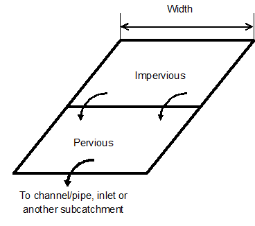
Figure 3-5 Re-routing of overland flow (Huber, 2001).
For a given subcatchment, schemes 1 and 2 are mutually exclusive, while scheme 3 can be combined with either 1 or 2 if desired. For internal re-routing, the fraction to be routed is a user-specified input parameter. When flows are re-routed in this manner, the re-routed flow is distributed uniformly over the downstream subarea or subcatchment, in the same manner as rainfall. The flow is also delayed at least one time step longer than it would have been without this extra routing.
The modified overland flow algorithm permits routing of flow from the impervious subarea over the pervious subarea of the subcatchment, or vice versa. In the first instance, runoff from a rooftop might flow over a lawn. In the second instance, runoff from a lawn might flow over a sidewalk. This option is especially useful for simulation of "low impact development" (LID) practices (Wright and Heaney, 2001; Wright et al., 2000; Lee, 2003).
By routing flow from one subcatchment to another subcatchment, buffer strips or riparian zones may be simulated. Inflow to the downstream subcatchment is distributed uniformly over the downstream subcatchment in the same manner as rainfall. This can be done because of the nonlinear reservoir flow routing method in which there is no spatial variation through the subcatchment. However, it also means that outflow from one subcatchment cannot be directed just to the pervious area of a downstream subcatchment that contains both pervious and impervious sub-areas.
If such routing were desired, the downstream subcatchment should be separated into two: a pervious subcatchment and an impervious subcatchment. There is no limit on the length of the overland flow "chain" that can be assembled. Outflow from the most downstream subcatchment will flow into a pipe or channel inlet (node), or directly to an outfall node, as usual.
To accommodate these options the computational scheme described in section 3.4 is modified as follows:
After the runoff from each of its subareas is computed, the total runoff reported for the subcatchment is the flow that actually exits the subcatchment. For example, if 100% of the impervious runoff was directed onto the pervious area, then the reported runoff for the subcatchment would consist only of the computed runoff from the pervious area.
Most study areas will require some level of discretization into multiple subcatchments in order to properly characterize the spatial variability in overland drainage pathways, surface properties, and connections into drainage pipes and channels. Discretization begins with the identification of drainage boundaries (drainage divides) using a topographic map, the location of major sewer inlets using a sewer system map, and the selection of channel/pipes to be simulated "downstream" in the model. In an urban area, drainage divides based strictly on topography might not apply, since the subsurface drainage network might transport water in a direction opposite to the surface gradient. Hence, drainage boundaries must be determined with the aid of both a topographic map and sewer plans.
For instance, consider the Fisk B Catchment in Portland, Oregon, shown in Figure 3-6 (Portland BES, 1996). The discretization relies upon both surface contours and invert slopes of the collection sewers. Additional detail of Subcatchments 8412 and 9412 (highlighted in Figure 3-6) is shown in Figure 3-7. The surface drainage in Subcatchment 9412 is to the south, but the pipe connecting junctions 412 and 712 drains north! If only the surface contours were considered a quite different catchment response to rainfall would result than what actually exists.
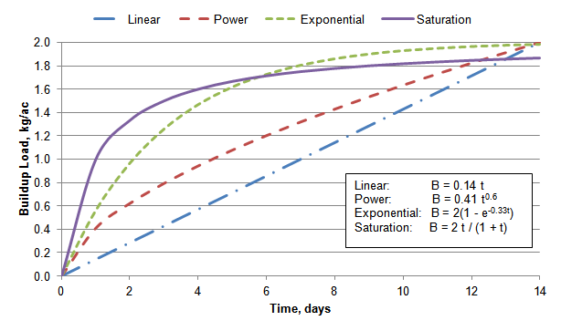
Figure 3-6 Fisk B catchment, Portland, Oregon (Portland BES, 1996).
Figure 3-7 Detailed view of two Fisk B subcatchments (Portland BES, 1996).
It is possible with SWMM to provide detail down to the parcel (individual lot) level, if desired and to simulate virtually every drainage pipe or channel (e.g., Huber and Cannon, 2002). The amount of detail actually required depends upon the purpose of the simulation. For screening purposes with continuous simulation, a coarse discretization with a few or just one subcatchment will generally suffice, with one or no channel/pipes. On the other hand, if hydraulic conditions are being studied within the catchment, enough detail in the drainage system and in the subcatchments that feed it must be provided. That is, obviously, a pipe must be simulated in order to study it, and every channel or pipe must have a source of inflow (subcatchment or channel/pipe) at the upstream end. The most upstream end of a series of channel/pipes must have a subcatchment draining to it or it will remain dry (and useless) during the simulation. If the principal interest is in flow at the outlet of the catchment, it is usually acceptable to provide minimal detail (e.g., few or one subcatchment and one or no channel/pipes). The trade-off, however, is that the coarser the schematization, the more decisions must be made on how to aggregate catchment properties.
For both single-event and continuous simulations, the amount of detail should be the minimum consistent with requirements for within-catchment information. Obviously, no information can be obtained about upstream surcharging if the upstream conduits are not simulated and subcatchments are not provided to feed them. In addition, sufficient detail needs to be provided to allow within-system control options to be tried for different areas and land uses. If, however, the primary objective is simply to produce a hydrograph and pollutograph at the outlet, using a single rain gage, then one subcatchment will often (but not always) serve as well as many.
Each subcatchment is schematized as in Figure 3-4, in which three sub-areas A1, A2, and A3 are used to represent different pervious and impervious surfaces. The slope of the idealized subcatchment is in the direction perpendicular to the flow width. The normal option is for outflow from each subarea to move directly to an inlet node of a drainage pipe or channel and not pass over any other subarea. That is, the impervious area is assumed to be directly connected impervious area (DCIA) or hydraulically effective impervious area. Rooftops or other surfaces that drain onto adjacent pervious areas are not directly connected and, if the user wishes, runoff from such non-DCIA surfaces may be directed to the pervious area of the subcatchment and vice versa. All sub-areas are assumed to have the same width perpendicular to the overland flow path. If desired, any subcatchment may consist entirely of any one (or more) types of the three subarea categories.
Actual subcatchments seldom exhibit the uniform rectangular geometries shown in Figure 3-4. In terms of runoff generation, all geometrical properties are merely parameters (as explained below) and no inherent "shape" can be assumed in the nonlinear reservoir technique. Parameter selection is aided with reference to Figure 3-2 and Equation 3-5 in which the subcatchment "reservoir" is shown in relation to inflows and outflows (or losses). Subcatchment outflow is a function of the coefficient \(\alpha = \frac{1.49WS^{1/2}}{A\ n}\) and the excess in ponded depth above depression storage. Note that the relative area A, width W, slope S, and roughness n are combined into the single parameter α. Equivalent changes in computed runoff may be caused by appropriate alteration of any of these parameters. Note also that the width and slope are the same for both the pervious and impervious subareas. Manning's roughness and relative area are the only parameters available to the modeler to characterize the relative contributions of pervious and impervious areas to the outlet hydrograph. (However, see further comments below on the subcatchment width.)
The following subsections discuss how values for subcatchment area, imperviousness, width, slope, roughness, and depression storage can be assigned and the implications they entail.
In principle, the catchment and subcatchment area can be defined by constructing drainage divides on topographic maps. In practice, this may or may not be easy because of the lack of detailed contour information and the presence of unknown inflows and outflows. This may be most noticeably brought to the modeler\'s attention when the measured runoff volume exceeds the measured rainfall volume, if the latter is correct. Actual storm rainfall is seldom accurately measured over all subcatchments.
From the modeling standpoint, there are no upper or lower bounds on subcatchment area. Subcatchments are usually chosen to coincide with different land uses, with drainage divides, and to ease parameter estimation, i.e., homogeneous slopes, soils, etc.
The percent imperviousness of a subcatchment is another parameter that can, in principle, be measured accurately from aerial photos or land use maps. In practice, unless impervious layers are included in a GIS representation of the basin, such work tends to be tedious, and it is common to make careful measurements for only a few representative areas and extrapolate to the rest. Runoff volume and flow rates are strongly sensitive to estimates of imperviousness; hence, care should be taken in imperviousness estimates.
One approach to estimating impervious area across large areas with multiple land uses is to associate a percent impervious area with each category of land use. Then by knowing the percentage of each land use within a subcatchment one can calculate its percentage impervious area. Table 3-1 lists estimates of percent impervious area for different land uses taken from EPA's Rouge River Project (Kluitenberg 1994) and incorporated into EPA technical guidance for MS4 stormwater permitting in Region I (US EPA, 2014).
Table 3-1 Impervious area as a percentage of land use.
| Land Use | Percent Impervious Area |
|---|---|
| Commercial | 56 |
| Industrial | 76 |
| High density residential | 51 |
| Medium density residential | 38 |
| Low density residential | 19 |
| Institutional | 34 |
| Agricultural | 2 |
| Forest | 1.9 |
| Open Urban Land | 11 |
As mentioned earlier, impervious areas in SWMM are hydraulically (directly) connected to the drainage system – called directly connected impervious areas (DCIA). For instance, if rooftops drain onto adjacent pervious lawn areas, they should not be treated as a hydraulically effective impervious area. Such areas are non-effective impervious areas (Doyle and Miller, 1980). On the other hand, if a driveway drains to a street and then to a stormwater inlet, the driveway would be considered hydraulically connected. Rooftops with downspouts connected directly to a sewer are clearly hydraulically connected. An example of careful measurements and statistics on imperviousness may be found in Field et al. (2000), Lee (2003), and Roy and Shuster (2007). Lee and Heaney (2003) provide detailed comparisons of imperviousness computations and their implications for modeling.
Should rooftops be treated as "pervious," the real surrounding pervious area is subject to more incoming water than rainfall alone and thus might produce runoff sooner than if rainfall alone were considered. In the possible event that this effect is important (a judgment based on infiltration parameters) it can be modeled using the overland flow re-routing option discussed earlier in Section 3.7. For example, if disconnected rooftops comprised 25 percent of the total impervious area of a subcatchment (as opposed to the total DCIA) then one could tell SWMM that this percentage of impervious area should be internally routed onto the pervious sub-area of the subcatchment.
Another method of estimating the effective impervious area given measured data is to plot the runoff (in. or mm) vs. rainfall (in. or mm) for small storms. The slope of the regression line is a good estimate of the effective impervious area (Doyle and Miller, 1980).
Southerland (2000) has proposed a series of regression equations relating effective impervious area (EIA) to total impervious area (TIA) based on data from over 40 sub-basins collected by the USGS in Oregon. Each equation has the form \(EIA = a{TIA}^{b}\) where the coefficients a and b are listed in Table 3-2. Further information on the concept of directly connected (or "hydraulically effective") impervious areas is contained in the review article by Shuster et al. (2005).
Table 3-2 Coefficients for Southerland's EIA equations.
| a | b | Condition |
|---|---|---|
| 0.1 | 1.5 | Average basins served by storm sewers and residential rooftops are not directly connected to sewers. |
| 0.4 | 1.2 | Highly connected basins with residential rooftops directly connected to storm sewers. |
| 1.0 | 1.0 | Totally connected basins that are completely served by storm sewers to which all impervious surfaces are directly connected. |
| 0.04 | 1.7 | Partly disconnected basins where more 50% of the area is served by grassy swales or roadside ditches instead of storm sewers and residential rooftops are not directly connected to sewers. |
| 0.01 | 2.0 | Highly disconnected basins where only a small percentage of area is served by storm sewers or has 70 percent or more draining to infiltration areas. |
If overland flow is visualized as running down-slope off of an idealized, rectangular catchment, then the width of the subcatchment is the physical width of overland flow. This may be seen for the idealized catchment shown once again in Figure 3-8 in which the lateral flow per unit width, q_L, is computed and multiplied by the width to obtain the total inflow into the channel. (As mentioned previously, the SWMM channel/pipes can only receive a concentrated inflow at their inlet nodes, however, and do not receive inflow distributed along their length.) Note also in Figure 3-8 that for this idealized case, if the two sides of the subcatchment are symmetrical the total width is twice the length of the drainage channel.
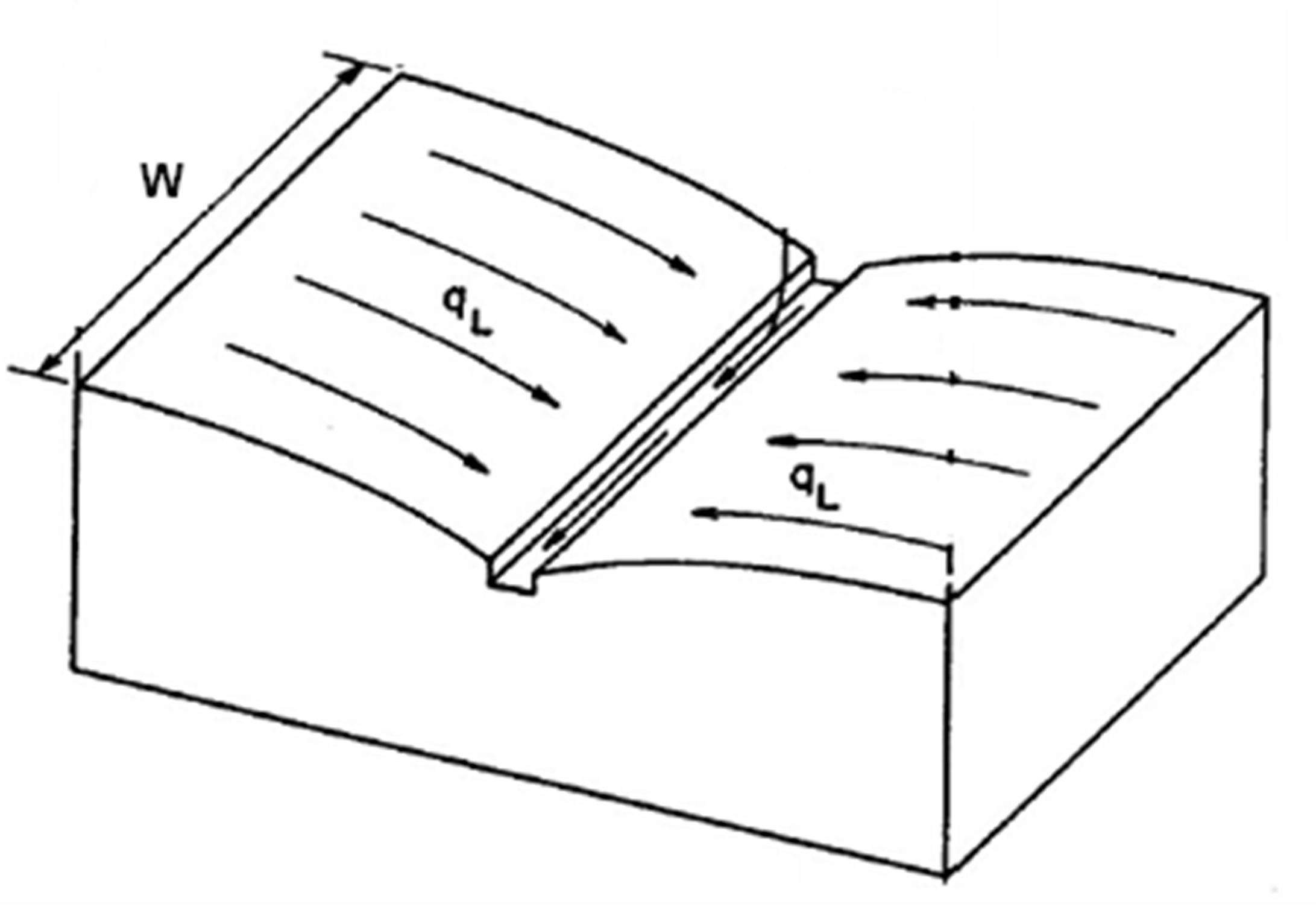
Figure 3-8 Idealized representation of a subcatchment.
Because real subcatchments will not be rectangular with properties of symmetry and uniformity, it is necessary to adopt other procedures to obtain the width for more general cases. This is of special importance because if the slope and roughness are fixed (see Equation 3-4), the width can be used to alter the hydrograph shape.
For example, consider the five different subcatchment shapes shown on Figure 3-9. Catchment hydraulic properties, routing parameters are given in Table 3-3. Outflow hydrographs for continuous rainfall and for rainfall of duration 20 min are shown on Figure 3-10. These were computed using the nonlinear reservoir equation (Section 3.1) with a time step of 5 min. Clearly, as the subcatchment width is narrowed (i.e., the outlet is constricted), the time to equilibrium outflow increases. Thus, equilibrium is achieved quite rapidly for cases A and B and more slowly for cases C, D and E.
Two routing effects may be observed. A storage effect is very noticeable, especially when comparing hydrographs A and E for duration of 20 minutes. The subcatchment thus behaves in the familiar manner of a reservoir. For case E, the outflow is constricted (narrow); hence, for the same amount of inflow (rainfall) more water is stored and less released. For case A, on the other hand, water is released rapidly and little is stored. Thus case A has both the fastest rising and recession limbs of the hydrographs.
A shape effect is also evident. Theoretically, all the hydrographs peak simultaneously (at the cessation of rainfall). However, a large width (e.g., case A) will cause equilibrium outflow to be achieved rapidly, producing a flat-topped hydrograph for the remainder of the (constant) rainfall. Thus, for a catchment schematized with several subcatchments and subject to variable rainfall, increasing the widths tends to cause peak flows to occur sooner. In general, however, shifting hydrograph peaks in time is difficult to achieve through adjustment of subcatchment flow routing parameters. The time distribution of runoff is by far most sensitive to the time distribution of rainfall.
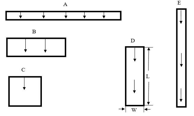
Figure 3-9 Rectangular subcatchments for illustration of shape and width effects.
Table 3-3 Data for example of effect of subcatchment width.
| Shape | A (ft²) | W (ft) | L (ft) |
|---|---|---|---|
| A | 40,000 | 800 | 50 |
| B | 40,000 | 400 | 100 |
| C | 40,000 | 200 | 200 |
| D | 40,000 | 100 | 400 |
| E | 40,000 | 50 | 800 |
Parameters: Slope = 1%, Imperviousness = 100%, Depression Storage = 0, n = 0.02, Equilibrium outflow = i*A = 0.926 cfs, ∆t = 5 min = 300 sec, i* = Rainfall excess = 1.0 in./hr = 0.000023148 ft/sec
Figure 3-10 Subcatchment hydrographs for different shapes of Figure 3-9.
So what is the best estimate of subcatchment width? If the subcatchment has the appearance of Figure 3-8, then the width is approximately twice the length of the main drainage channel through the catchment. However, if the drainage channel is on the side of the catchment as in Figure 3-9, the width is just the length of the channel. A good estimate for the width can be obtained by determining the average maximum length of overland flow and dividing the area by this length.
For example, consider Subcatchment 8412 of the Fisk B Catchment, shown in Figure 3-7. The area of Subcatchment 8412 is approximately 72,820 ft2 (1.67 ac). A crude estimate of the average distance from the street to the drainage divide for overland flow is made by measuring the length on the map ten times (Table 3-4). The street in the lower part of the subcatchment is divided into six equal segments, approximately 57 ft in length. Distances to the boundary (drainage divide) from the centerline of the street are then measured normal to the contours from each of the five internal locations along the street:
The width is then estimated as W ≈ 72,820 / 119 = 612 ft. Clearly, the average length estimate can be improved with several additional measurements off the figure. But in practice, this may even be done "by eye," since width is sometimes used as a calibration parameter. The distances are measured to each side of the street under the assumptions that travel times along the street are much less than off the lots. This may not be true if roof drains are directly connected to the street (unknown for this example).
Table 3-4 Width computations for Portland example.
| North side of street to boundary (ft) | South side of street to boundary (ft) |
|---|---|
| 247 | 31 |
| 247 | 74 |
| 232 | 74 |
| 103 | 74 |
| 74 | 60 |
| Sum: 1,186 ft; Average: 119 ft |
When assigning an overland flow path length, particularly for sites with natural land cover, one must recognize that there is a maximum distance over which true sheet flow prevails. Beyond this, runoff consolidates into rivulet flow with much faster travel times and less opportunity for infiltration. There is no general agreement on what distance should be used as a maximum overland flow path length. The Natural Resources Conservation Service recommends a maximum length of 100 ft (NRCS, 2010) while Denver's Urban Drainage and Flood Control District uses a maximum of 500 ft. (UDFCD, 2007).
Another estimate for the width is twice the length of the main drainage channel, the street in this instance. The street is approximately 360 ft long, which would give an estimate of about 720 ft for the Subcatchment
However, this estimate assumes approximately equal areas on both sides of the drainage channel whereas most real subcatchments will be irregular in shape and have a drainage channel that is off center, as in Figure 3-11. This is especially true of rural or undeveloped catchments. A simple way of handling this case is given by DiGiano et al. (1977). A skew factor may be computed,
\[Z = \frac{A_{m}}{A}\]
(3-10)
where:
Z = skew factor, 0.5 ≤ Z ≤ 1,
A*_m_* = larger of the two areas on each side of the channel
A = total area.
Figure 3-11 Irregular subcatchment shape for width calculations (DiGiano et al., 1977, p. 165).
If L is the length of the main drainage channel then the width W is simply weighted sum between the two limits of L and 2L:
\[W = L + 2L(1 - Z)\]
(3-11)
Applying this idea to Subcatchment 8412 of Figure 3-7, the area north of the street centerline is approximately 1.19 ac, and the area of the street and south is approximately 0.48 ac. Hence,
Z = 1.19 / 1.67 = 0.71
and an estimate for the width is,
W = 360 + 2 × 360 × (1 - 0.71) = 567 ft
This estimate is not far from the estimate of roughly 610 ft obtained by dividing the area by the average maximum flow length.
A more fundamental approach to estimating both subcatchment width and slope has recently been developed by Guo and Urbonas (2007). The idea is to use "shape factors" to convert a natural watershed as pictured in Figure 3-11 into the idealized overland flow plane of Figure 3-8. A shape factor is an index that reflects how overland flows are collected in a watershed. The shape factor X for the actual watershed is defined as \(\frac{A}{L^{2}}\) where A is the watershed area and L is the length of the watershed's main drainage channel (not necessarily the length of overland flow). The shape factor Y for the idealized watershed is \(W/L\). Requiring that the areas of the actual and idealized watersheds be the same and that the potential energy in terms of the vertical fall along the drainage channel be preserved, Guo and Urbonas (2007) derive the following expression for the shape factor Y of the idealized watershed:
\[Y = 2X(1.5 - Z)(2K - X)/(2K - 1)\]
(3-12)
where K is an upper limit on the watershed shape factor. Guo and Urbonas (2007) recommend that K be between 4 and 6 and note that a value of 4 is used by Denver's Urban Drainage and Flood Control District. Once Y is determined, the equivalent width W for the idealized watershed is computed as \(YL\).
Applying this approach to Subcatchment 8412 (using K = 4) produces the following:
X = (1.67 acres × 43,560 ft²/acre) / (360²) = 0.56
Z = 1.19 / 1.67 = 0.71
Y = (2 × 0.56) × (1.5 - 0.71) × (0.56 - 2×4) / (1 - 2×4) = 0.94
W = 360 × 0.94 = 338 ft.
This width value is considerably lower than those derived from direct estimates of either the longest flow path length or the drainage channel length. As a result, it would most likely produce a longer time to peak for the runoff hydrograph.
To reiterate, changing the subcatchment width changes the routing parameter *α* of Equation 3-5. Thus, identical effects to those discussed above may be created by appropriate variation of the roughness and/or slope.
The subcatchment slope should reflect the average slope along the pathway of overland flow to inlet locations. For a simple geometry (e.g., Figures 3-8 and 3-9) the calculation is simply the elevation difference divided by the length of flow. For more complex geometries, several overland flow pathways may be delineated, their slopes determined, and a weighted slope computed using a path-length weighted average. Such a procedure is described by DiGiano et al. (1977, pp. 101-102).
Alternatively it may be sufficient to assume that overland flow occurs along what the user considers to be the hydrological dominant slope for the conditions being simulated. One would then choose the appropriate overland flow length, slope, and roughness for this equivalent plane. The Guo and Urbonas (2007) Shape Factor approach discussed in the previous section computes the slope of this equivalent plane as \(\frac{S_{o}L}{(A/YL + YL)}\) where S~o~ is the slope of the drainage channel and the other variables are as defined in Section 3.8.4.
Finally, if there are clearly two different slopes to consider for the subcatchment, it may be subdivided into two subcatchments and the overland flow re-routing option be used to route flow from the upper subcatchment onto the lower subcatchment.
Values of Manning's roughness coefficient, n, are not as well known for overland flow as for channel flow because of the considerable variability in landscape features, transitions between laminar and turbulent flow, very small flow depths, etc. Most studies indicate that for a given surface cover, n varies inversely in proportion to depth, discharge or Reynold's number. Such studies may be consulted for guidance (e.g., Petryk and Bosmajian, 1975; Chen, 1976; Christensen, 1976; Graf and Chun, 1976; Turner et al., 1978; Emmett, 1978), or generalized values used (e.g., Chow, 1959; Crawford and Linsley, 1966; Huggins and Burney, 1982; French, 1985; Engman, 1986; Yen, 2001).
Roughness values used in the Stanford Watershed Model (Crawford and Linsley, 1966) are given in Table 3-5 along with values from Engman (1986) and Yen (2001). Engman also provides values for other agricultural land uses and a good literature review. There is no consensus among the three sources of data in the table, reflecting the uncertainty in these estimates. However, recall the discussion of Equation 3-5 in Section 3.8.1. For SWMM, it is common to fix estimates of slope and Manning's n and calibrate with the subcatchment width.
Depression (retention) storage (depth d_S in Figure 3-2) is a volume that must be filled prior to the occurrence of runoff on both pervious and impervious areas (Viessman and Lewis, 2003). It represents a loss or "initial abstraction" caused by such phenomena as surface ponding, surface wetting, interception and evaporation. In the SWMM rainfall-runoff algorithm (Section 3.1), water stored as depression storage on pervious areas is subject to infiltration (and evaporation), so that available storage capacity is continuously and rapidly replenished. Water stored in depression storage on impervious areas is depleted only by evaporation and therefore it takes much longer to restore such storage to its full capacity.
| Source | Ground Cover | n | Range |
|---|---|---|---|
| Crawford and Linsley (1966)ᵃ | Smooth asphalt | 0.01 | |
| Asphalt of concrete paving | 0.014 | ||
| Packed clay | 0.03 | ||
| Light turf | 0.20 | ||
| Dense turf | 0.35 | ||
| Dense shrubbery and forest litter | 0.4 | ||
| Engman (1986)ᵇ | Concrete or asphalt | 0.011 | 0.010-0.013 |
| Bare sand | 0.010 | 0.01-0.016 | |
| Graveled surface | 0.02 | 0.012-0.03 | |
| Bare clay-loam (eroded) | 0.02 | 0.012-0.033 | |
| Range (natural) | 0.13 | 0.01-0.32 | |
| Bluegrass sod | 0.45 | 0.39-0.63 | |
| Short grass prairie | 0.15 | 0.10-0.20 | |
| Bermuda grass | 0.41 | 0.30-0.48 | |
| Yen (2001)ᶜ | Smooth asphalt pavement | 0.012 | 0.010-0.015 |
| Smooth impervious surface | 0.013 | 0.011-0.015 | |
| Tar and sand pavement | 0.014 | 0.012-0.016 | |
| Concrete pavement | 0.017 | 0.014-0.020 | |
| Rough impervious surface | 0.019 | 0.015-0.023 | |
| Smooth bare packed soil | 0.021 | 0.017-0.025 | |
| Moderate bare packed soil | 0.030 | 0.025-0.035 | |
| Rough bare packed soil | 0.038 | 0.032-0.045 | |
| Gravel soil | 0.032 | 0.025-0.045 | |
| Mowed poor grass | 0.038 | 0.030-0.045 | |
| Average grass, closely clipped sod | 0.050 | 0.040-0.060 | |
| Pasture | 0.055 | 0.040-0.070 | |
| Timberland | 0.090 | 0.060-0.120 | |
| Dense grass | 0.090 | 0.060-0.120 | |
| Shrubs and bushes | 0.120 | 0.080-0.180 | |
| Business land use | 0.022 | 0.014-0.035 | |
| Semi-business land use | 0.035 | 0.022-0.050 | |
| Industrial land use | 0.035 | 0.020-0.050 | |
| Dense residential land use | 0.040 | 0.025-0.060 | |
| Suburban residential land use | 0.055 | 0.030-0.080 | |
| Parks and lawns | 0.075 | 0.040-0.120 |
ᵃObtained by calibration of Stanford Watershed Model.
ᵇComputed by Engman (1986) by kinematic wave and storage analysis of measured rainfall-runoff data.
ᶜComputed on basis of kinematic wave analysis.
Depression (retention) storage (depth d_S in Figure 3-2) is a volume that must be filled prior to the occurrence of runoff on both pervious and impervious areas (Viessman and Lewis, 2003). It represents a loss or "initial abstraction" caused by such phenomena as surface ponding, surface wetting, interception and evaporation. In the SWMM rainfall-runoff algorithm (Section 3.1), water stored as depression storage on pervious areas is subject to infiltration (and evaporation), so that available storage capacity is continuously and rapidly replenished. Water stored in depression storage on impervious areas is depleted only by evaporation and therefore it takes much longer to restore such storage to its full capacity.
Depression storage may be used to simulate interception, the storage of rainfall on vegetation. Perhaps counter-intuitively, a tree, for instance, that intercepts rainfall can be simulated as an impervious surface, with depression storage (interception), whose runoff is onto an adjacent or underlying pervious surface. In this way, the interception capacity is regenerated only by evaporation.
As described earlier, a percent "*% Zero-Imperv*" of the impervious area is assigned zero depression storage in order to promote immediate runoff. Another option to achieve zero depression storage on impervious areas (and thus immediate runoff) is to set % Zero-Imperv to zero, and enter zero values for depression storage for the impervious area of each subcatchment, as desired.
Depression storage may be derived from rainfall-runoff data for impervious areas by plotting runoff volume V (depth) as the ordinate against rainfall volume P as the abscissa for several storms. The rainfall intercept at zero runoff is the depth of depression storage d_s, i.e., a regression of the form
\[V = C\left( P - d_{S} \right)\]
(3-13)
where C is a coefficient. This kind of analysis tends to work better for longer averaging periods than individual storm events, but for storm events will work better for small, more impervious catchments than for larger mixed catchments. The reason is that even for small rainfall amounts, impervious surfaces (DCIA) will generate some runoff (one reason for the % Zero-Imperv parameter). Hence, a depression storage value found as the intercept may be appropriate for a longer term water balance than for simulation of hydrographs.
Data obtained in this manner from 18 urban European catchments (Falk and Niemczynowicz, 1978, Kidd, 1978a, Van den Berg, 1978) showed that depression storages ranged between 0.005 and 0.059 inches, depending on slope, with an average of 0.023 inches. Kidd (1978b) presented the following regression for these data:
\[d_{S} = 0.303S^{0.49}\]
(3-14)
where d_s is depression storage (inches) and S is catchment slope (percent).
Viessman and Lewis (2003, p. 140) present a linear relation between depression storage and slope based on four small impervious areas near Baltimore, MD:
\[d_{S} = 0.136 - 0.032S\]
(3-15)
where the observed values of d_s ranged from 0.06 to 0.11 inches.
Separate values of depression storage can be used for the pervious and impervious subareas within a subcatchment. Representative values for the latter can probably be obtained from the European data just discussed. Pervious area measurements are lacking; most reported values are derived from successful simulation of measured runoff hydrographs. Although pervious area values are expected to exceed those for impervious areas, it must be remembered that the infiltration loss, often included as an initial abstraction in simpler models, is computed explicitly in SWMM. Hence, pervious area depression storage might best be represented as an interception loss, based on the type of surface vegetation. Many interception estimates are available for natural and agricultural areas (Linsley et al., 1949; Maidment, 1993; Viessman and Lewis, 2003). For grassed urban surfaces a value of 0.10 inches (2.5 mm) may be appropriate.
As mentioned earlier, several studies have determined depression storage values in order to achieve successful modeling results. For instance, Hicks (1944) in Los Angeles used values of 0.20, 0.15 and 0.10 inches (5.1, 3.8, 2.5 mm) for sand, loam and clay soils, respectively, in the urban area. Tholin and Keifer (1960) used values of 0.25 and 0.0625 inches (6.4 and 1.6 mm) for pervious and impervious areas, respectively, for their Chicago hydrograph method. Brater (1968) found a value of 0.2 inches (5.1 mm) for three basins in metropolitan Detroit. Miller and Viessman (1972) give an initial abstraction (depression storage) of between 0.10 and 0.15 inches (2.5 and 3.8 mm) for four composite urban catchments. The American Society of Civil Engineers (1992) suggests depression storage of 1/16 inch for impervious areas and 1/4 inch for pervious areas. The Denver Urban Drainage and Flood Control District (UDFCD, 2007) recommends depression storage losses of 0.1 inches for large paved areas and flat roofs, 0.05 inches for sloped roofs, 0.35 inches for lawn grass, and 0.4 inches for open fields.
In SWMM, depression storage may be treated as a calibration parameter, particularly to adjust runoff volumes. If so, extensive preliminary work to obtain an accurate a priori value may be unnecessary since the value will be changed during calibration anyway. Depression storage is most sensitive for small storms; as the depth increases it becomes a smaller and smaller relative component of the water budget.
Sensitivity of surface runoff volume and peak flow estimates to key surface runoff parameters is listed in Table 3-6. The influence of storm depth is not represented in the table.
Table 3-6 Sensitivity of runoff volume and peak flow to surface runoff parameters.
| Parameter | Typical effect on hydrograph | Effect of increase on runoff volume | Effect of increase on runoff peak | Comments |
|---|---|---|---|---|
| Area | Significant | Increase | Increase | Less effect for a highly porous catchment |
| Imperviousness | Significant | Increase | Increase | Less effect when pervious areas have low infiltration capacity. |
| Width | Affects shape | Decrease | Increase | For storms of varying intensity, increasing the width tends to produce higher and earlier hydrograph peaks, a generally faster response. Only affects volume to the extent that reduced width on pervious areas provides more time for infiltration. |
| Slope | Affects shape | Decrease | Increase | Same as for width, but less sensitive, since flow is proportional to square root of slope. |
| Roughness | Affects shape | Increase | Decrease | Inverse effect as for width. |
| Depression storage | Moderate | Decrease | Decrease | Significant effect only for low-depth storms. |
Losses (ET, depression storage, infiltration) are relatively less important as the storm depth increases. That is, for flooding the land surface behaves more and more like an impervious surface, which is one reason why urbanization has less impact on high-return period events than on common events. If ground saturation is an important consideration, then the groundwater routines (Chapter 5) might be invoked to allow the water table to rise to the surface, or the maximum infiltration volume option used (Chapter 4). When calibrating for more common (lower depth) events, depression storage becomes more important, especially as the storm depth drops to just a few tenths of an inch. Calibration for small storms is often difficult, since depression storage is difficult to estimate and dependent on initial conditions.
Earlier in section 3.8.4 a numerical example was presented showing the effect that the width parameter had on the runoff hydrographs from a completely impervious subcatchment subjected to constant rainfall intensity. This section presents a more realistic example that highlights the difference in runoff responses between impervious and pervious subcatchments that are subjected to the same design storm hyetograph. Table 3-7 lists the parameters used for each subcatchment. Note that normally a single subcatchment could be used to contain both of these sub-areas, but they are represented here as separate subcatchments so that the runoff from each can be compared more readily.
| Item | Parameter | Impervious Subcatchment | Pervious Subcatchment |
|---|---|---|---|
| Subcatchment | Area (acres) | 5 | 5 |
| Percent Impervious | 100 | 0 | |
| Percent Slope | 0.5 | 0.5 | |
| Width (ft) | 140 | 140 | |
| Roughness | 0.01 | 0.1 | |
| Depression Storage (in) | 0.05 | 0.05 | |
| Percent with No Depression Storage | 25 | 0 | |
| Evaporation (in/hr) | 0 | 0 | |
| Horton Infiltration | Initial Capacity (in/hr) | N/A | 1.2 |
| Final Capacity (in/hr) | N/A | 0.1 | |
| Decay Coefficient (hr^-1^) | N/A | 2.0 | |
| Design Storm | Duration (hr) | 6.0 | 6.0 |
| Total Depth (in) | 2.0 | 2.0 | |
| Time-to-Peak / Duration | 0.375 | 0.375 |
The two subcatchments were given identical area, slope, width, and depression storage. The roughness of the pervious subcatchment was made ten times higher than the impervious roughness as reflected in Table 3-7. The infiltration parameters for the pervious area are representative of a well-drained sandy loam soil. A description of the Horton infiltration method used in SWMM is supplied in the next chapter. The design storm is a 6-hour, 2-inch event with a triangular-shaped hyetograph.
Table 3-7 Parameters used for illustrative runoff example
| Item | Parameter | Impervious Subcatchment | Pervious Subcatchment |
|---|---|---|---|
| Subcatchment | Area (acres) | 5 | 5 |
| Percent Impervious | 100 | 0 | |
| Percent Slope | 0.5 | 0.5 | |
| Width (ft) | 140 | 140 | |
| Roughness | 0.01 | 0.1 | |
| Depression Storage (in) | 0.05 | 0.05 | |
| Percent with No Depression Storage | 25 | 0 | |
| Evaporation (in/hr) | 0 | 0 | |
| Horton Infiltration | Initial Capacity (in/hr) | N/A | 1.2 |
| Final Capacity (in/hr) | N/A | 0.1 | |
| Decay Coefficient (hr^-1^) | N/A | 2.0 | |
| Design Storm | Duration (hr) | 6.0 | 6.0 |
| Total Depth (in) | 2.0 | 2.0 | |
| Time-to-Peak / Duration | 0.375 | 0.375 |
Figure 3-12 shows the runoff hydrographs that result for the example design event. Flow rates are represented on a per unit area basis so that they can be compared against the rainfall intensities. For the impervious area, runoff from the 25% of the area with no depression storage begins immediately, while runoff from the remaining area is delayed by the available depression storage at the start of the storm. After this storage is filled, the impervious runoff hydrograph follows that of the storm hyetograph. About 97% of the rain that falls on the impervious area becomes runoff and there is a slight reduction in peak runoff rate. For the pervious area there is no runoff at all for the first 2 hours of the storm, as the depression storage and available infiltration capacity are sufficient to capture all of the rainfall volume during this period. After this, the remaining infiltration capacity is such that only 30% of the total storm volume becomes runoff. The peak runoff rate is only one third of the peak rainfall rate. When taken together, the total hydrograph (equal to half the sum of the two sub-area hydrographs, since flows are expressed per unit area) reduces the peak storm intensity by 50% and the total storm volume by 64%.
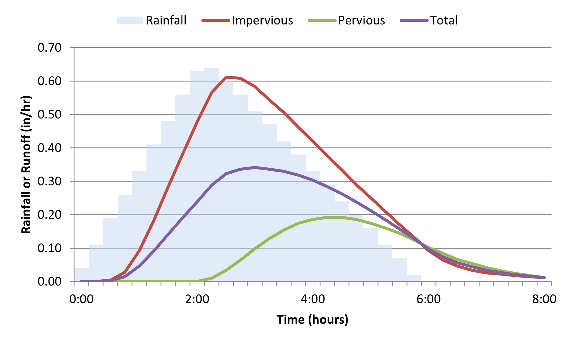
Figure 3-12 Runoff results for illustrative example.
To varying degrees it is possible to have the results of SWMM's runoff computations approximate those obtained from other well known methods. The following sub-sections describe how to do this for the runoff coefficient method, the SCS Curve Number method, and the unit hydrograph method.
This method is sometimes used in preliminary screening-level models to generate runoff flows from long-term rainfall records or rainfall probability distributions with a minimum of site-specific data required (see STORM (Corps of Engineers, 1977); NetSTORM (Heineman, 2004); Adams and Papa, 2000). It computes runoff Q (cfs) after all depression storage has been filled as:
\[Q = CiA\]
(3-16)
where C is a runoff coefficient, i is the rainfall rate (ft/s), and A is the subcatchment area (ft2). If infiltration over the pervious area is considered then
\[Q = \left\lbrack Ci + (1 - C)max(0,\ i - f) \right\rbrack A\]
(3-17)
where f is a constant infiltration rate (ft/s) and C can be interpreted as the fraction of impervious area. Values of C have been tabulated for various types of land uses (see ASCE, 1992 or UDFCD, 2007).
To implement this approach in SWMM one could do the following:
Setting up a model in this fashion will produce exactly the same results as if Equations 3-16 or 3-17 were implemented directly. When the Manning roughness n is 0, SWMM bypasses Equation 3-1 and simply converts all rainfall excess at each time step into instantaneous runoff.
Note that this method completely ignores any storage or delay that overland flow contributes to the shape of a runoff hydrograph as well as the declining rate of infiltration that occurs over time. It can, however, allow one to perform preliminary screening types of analyses relatively quickly with a minimum of site data required.
The SCS (Soil Conservation Service, now known as the Natural Resources Conservation Service) Curve Number method is a widely used procedure for computing runoff from single-event design storms. As implemented in NRCS's TR-55 manual (NRCS, 1986) it consists of three separate runoff–related computations: one computes total runoff volume for any given rainfall event while the other two estimate a peak discharge and a runoff hydrograph for a synthetic 24-hour design storm with a given return period. These latter two computations utilize a kinematic wave approach to overland flow as well as a standard 24-hour design storm time distribution and are therefore incompatible with SWMM's approach to generating runoff hydrographs. SWMM can however, approximate the Curve Number method's estimate of total runoff volume from a subcatchment by doing the following:
As an example, consider a residential area with a Curve Number of 80 subjected to a uniform storm of 4 inches over 4 hours. The SCS method for computing runoff volume (for US units) is:
\[R = \frac{(P - Ia)^{2}}{P - Ia + S}\]
(3-18)
where
\[S = \frac{1000}{CN} - 10\]
(3-19)
and
R = cumulative runoff volume (inches)
P = cumulative rainfall (inches)
Ia = initial abstraction (inches)
S = soil moisture storage capacity (inches)
CN = curve number
Using the SCS recommended initial abstraction of 0.2S = 0.5 inches, the resulting SCS runoff volume is 2.04 inches. Running SWMM for a single subcatchment in the manner prescribed above produces a total runoff volume of 1.98 inches. When a roughness of 0.1 (along with a width of 100 ft and slope of 0.5%) is used to allow SWMM to produce a more realistic runoff hydrograph, the total runoff volume drops to 1.67 inches due to the increased time available for ponded water to infiltrate as it flows over the surface.
A unit hydrograph (UH) is a linear transfer function used to convert a time series of rainfall excess into a runoff hydrograph. A unit hydrograph can be derived from observed rainfall-runoff records within a specific catchment or be chosen from a number of synthetic unit hydrographs that have been developed over the years. The shapes of synthetic hydrographs have been parameterized with respect to certain geographic and land cover variables. Specific examples include Snyder's UH, Clark's UH, the Espey-Altman UH, the SCS (NRCS) Dimensionless UH, the SCS (NRCS) Triangular UH, the Santa Barbara Urban Hydrograph, and the Colorado Urban Hydrograph (see Nicklow et al, 2006 for further details). As an example, the SCS (NRCS) triangular UH is shown in Figure 3-13. The parameters Q_p and t_p are functions of the catchment's time of concentration and its area.

Figure 3-13 SCS (NRCS) triangular unit hydrograph (NRCS, 2007).
SWMM normally uses a unit hydrograph approach to empirically model the process by which rainfall causes subsurface inflow into leaky sewer pipes, otherwise known as rainfall dependent inflow/infiltration (RDII). The details are described in Chapter 7. Any location within the drainage system can have a set of RDII UH's assigned to it. Each set of UH's can consist of up to three individual triangular UH's (like the one shown in Figure 3-13). One can therefore use an RDII-type analysis to replace SWMM's normal rainfall-runoff computational scheme by doing the following:
After running SWMM with these modifications, the runoff hydrographs for each subcatchment are equivalent to the Lateral Inflow results produced at each subcatchment's outlet node.
There are clearly some limitations to keep in mind when considering this approach. First, SWMM can only utilize triangular shaped unit hydrographs. This might require some approximation if one wishes to use one of the standard synthetic unit hydrographs whose shape is not triangular. Second, any losses from infiltration must be taken into account when the unit hydrographs are constructed. SWMM's RDII procedure does not account for the details of soil infiltration in the manner that SWMM's normal runoff modeling does. Finally, in by-passing SWMM's normal runoff procedure one also loses the ability to model other subcatchment-related phenomena, such as overland flow re-routing as described in section 3.7 or pollutant buildup and washoff.
Finally, it should be mentioned that it is possible to use any set of externally generated runoff data to drive SWMM's flow and pollutant routing routines. This can be done by placing the runoff time series data in a specially formatted Routing Interface file. This is a text file whose format is described in the SWMM 5.0 Users Manual (EPA, 2013). An excerpt from such a file that supplies runoff hydrographs to two nodes within a drainage network is reproduced in Table 3-8. A Routing Interface file can be used in lieu of defining any subcatchments and rainfall data for a study area. Or it can be used as a replacement for the runoff that would have been generated by SWMM for the subcatchments and rainfall data already defined for the study area. In this case SWMM's Ignore Rainfall/Runoff option must be invoked to prevent the program from adding any internally computed runoff to that being provided by the interface file.
Table 3-8 Contents of a typical Routing Interface file
| File Entry | Remarks |
|---|---|
| SWMM5 | Required identifier |
| Example File | Data file description (can be blank) |
| 300 | Time step for all data (seconds) |
| 1 | Number of variables provided by the file |
| FLOW CFS | Name and units of each variable (one per line) |
| 2 | Number of nodes with inflow data |
| N1 | Name of each node (one per line) |
| N2 | |
| Node Year Mon Day Hr Min Sec Flow | Column headings for data to follow (can be blank) |
| N1 2002 04 01 00 20 00 0.000000 | Node, year, month, day, hour, minute, second, and value for each time step |
| N2 2002 04 01 00 20 00 0.002549 | |
| N1 2002 04 01 00 25 00 0.000000 | |
| N2 2002 04 01 00 25 00 0.002549 | |
| etc. |
 1.13.2