Problem

A constituent enters a network and has to be carried through it. Every transport engine answers the same question — what concentration is where, when — and they disagree most where a model usually cares most: at a front.

[OPTIONS] QUALITY_SOLVER chooses between three. The legacy engine treats each conduit as a stirred tank. The Eulerian engine cuts the conduit into cells and advects with a flux-limited scheme. The Lagrangian engine carries parcels of water that keep their concentration until they mix. This chapter sends one step of conservative tracer through all three.

Deck

Deck: docs/figures/decks/transport_demo/transport_demo.inp

Five junctions in a line discharging to an outfall through five 100 m conduits. A constant 0.2 m³/s inflow enters at J1 from t = 0 carrying a conservative tracer at 10 mg/L, a first-order decaying constituent at 20 mg/L and an inlet temperature of 18 °C. Because the inflow starts into a clean system, the tracer arrives at each junction as a step.

The deck is the SWMMVis tutorial's transport demonstration, with four process components configured from sidecar files. The same deck carries Chapter 9 and Chapter 10.

Options that select the formulation

[OPTIONS]
FLOW_UNITS           CMS
INFILTRATION         HORTON
FLOW_ROUTING         DYNWAVE
START_DATE           01/01/2026
START_TIME           00:00:00
END_DATE             01/01/2026
END_TIME             06:00:00
REPORT_STEP          0:05:00
ROUTING_STEP         5
QUALITY_SOLVER       EULERIAN_ARD
WATER_AGE            ON
HEAT_TRANSPORT       ON

and the inflows that make the front:

[INFLOWS]
;;Node  Constituent      TimeSeries  Type    Mfactor  Sfactor  Baseline
J1      FLOW             ""          FLOW    1.0      1.0      0.2
J1      TRACER           ""          CONCEN  1.0      1.0      10.0
J1      DECAY            ""          CONCEN  1.0      1.0      20.0
J1      __TEMPERATURE__  ""          CONCEN  1.0      1.0      18.0

The Eulerian engine's own options live in the component's sidecar rather than in the deck, which is where TARGET_DX is set:

[TRANSPORT_OPTIONS]
DISPERSION      FISCHER
SCALAR_SCHEME   MUSCL
LIMITER         VANLEER
TARGET_DX       25

One caution about reporting. The deck reports every five minutes, and the front crosses the whole line in about five minutes: at that resolution every engine looks identical because the report steps over the event. The figures below upsert REPORT_STEP 0:00:10. If a comparison of engines looks like no difference at all, check the reporting step before concluding anything.

Results

Figure 8-1

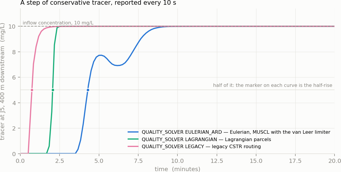
Figure 8-1 A step of conservative tracer at the downstream junction under the three transport engines

`QUALITY_SOLVER`	Half-rise at J5	Plateau	Run time
`LEGACY`	0.74 min	10.000 mg/L	0.05 s
`LAGRANGIAN`	2.05 min	10.000 mg/L	0.15 s
`EULERIAN_ARD`	4.29 min	10.000 mg/L	0.12 s

Table 8-1 When half the inflow concentration reaches J5, 400 m downstream

All three conserve mass and all three reach the same plateau. The disagreement is entirely about when, and it is large: the legacy engine has half the concentration at J5 within 45 seconds, the Eulerian engine not for four and a half minutes. A tracer study calibrated against one of these would be badly wrong under another.

Why the legacy engine is early. A stirred tank has no travel time. Mass entering a conduit is instantly available at its downstream end in proportion to the volume ratio, so a front propagates through the network as fast as the mixing cascade allows rather than as fast as the water moves. For a long-duration load — a continuous discharge, a storm's worth of washoff — the difference integrates away, which is why this engine remains the default and remains adequate for most quality work.

Why the Lagrangian engine is between them. Parcels move with the water, so the arrival is the water's arrival. The rise is nearly vertical because a parcel keeps its concentration: what smears the front is the mixing at each junction, not the advection.

Why the Eulerian engine is latest, and not simply diffusive. It advects on a fixed mesh with a limited second-order scheme, so the front arrives with the water and is spread by the dispersion term rather than by the scheme. The dip near six minutes is the node-by-node structure of the line showing through: each junction mixes what has arrived so far, and with dispersion turned on the reach behind the front is still filling.

`TARGET_DX`: what refinement buys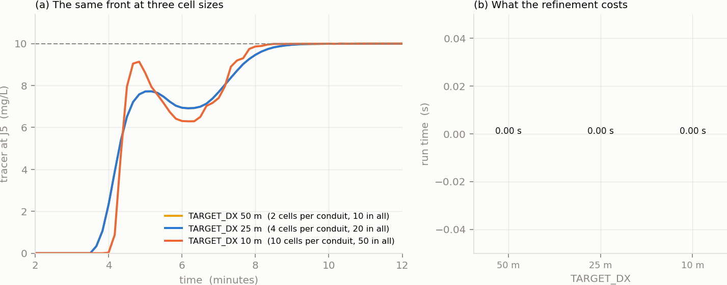

Figure 8-2

Figure 8-2 The same front under the Eulerian engine at three cell sizes, and what each costs

`TARGET_DX`	Cells per conduit	Half-rise at J5	Run time
50 m	2	4.29 min	0.10 s
25 m	4	4.29 min	0.12 s
10 m	10	4.35 min	0.17 s

Table 8-2 The Eulerian engine at three cell sizes on the same deck

The arrival time is already converged at two cells per conduit; what refinement changes is the sharpness of the front. The 10 m run rises almost vertically and overshoots to 9.2 mg/L before settling, where the coarser runs round the corner off. That overshoot is the limiter working at a discontinuity, not an instability, and it is bounded by the neighbouring values.

Refinement is quadratic in cost in general — halving TARGET_DX doubles both the cell count and the substep count — though on a deck this small the constant overhead dominates and the ratio is only 1.7×. On a network model the quadratic term is the one that matters.

Where to go next