Chapter 6: Building a Coupled One- and Two-Dimensional Model

Problem

A one-dimensional model reports water leaving a node as flooding, and then loses it. For a capacity assessment that is enough. For a flood map, an evacuation route or a depth at a doorway, it is not: the question is where the water goes, how deep it gets, and when it comes back.

Adding a mesh answers that, and adds three things to get right — the mesh, the boundaries, and the coupling between the two solvers. This chapter builds all three on the engine's own complete example.

Deck

Deck: docs/figures/decks/coupled_1d2d/2d_complete_example.inp

A deliberately small model: a 1D network of junctions, a storage unit and an outfall, beside a mesh of eight triangles over nine vertices. It is small so that every feature is visible at once — five boundary-condition types, both kinds of coupling point, per-edge conveyance factors — rather than realistic.

The 2D results go to an HDF5 file named by the deck, and both figures on this page are read from it.

Options that select the formulation

The mesh itself is [2D_VERTICES] and [2D_TRIANGLES]; the solver is configured in [2D_OPTIONS]:

[2D_OPTIONS]
MAX_TIMESTEP            10.0       ;; caps the marcher step and the sync batch
DRY_DEPTH               0.001      ;; wet/dry threshold
COUPLING_CD             0.65       ;; default discharge coefficient
INTEGRATOR              EXPLICIT   ;; the explicit local-inertial marcher
CFL_NUMBER              0.7
H_MOVE                  0.003      ;; below this a cell is integrated lazily
LTS_TIERS               4          ;; local time stepping tiers
COUPLING_AREA           DEFAULT
REPORT_2D               YES
OUTPUT_FILE             2d_complete_example.h5

The momentum closure is the one key this chapter varies:

MOMENTUM_EQUATION       LOCAL_INERTIAL    ;; or FULL_SWE, or DIFFUSIVE_WAVE

Coupling is declared in two ways, and they mean different things.

[2D_VERTEX_NODE_MAP]
;; VERTEX  SWMM_NODE  CD     AREA
   4       J1         0.65   2.0
 
[2D_TRIANGLE_NODE_MAP]
;; TRIANGLE_OR_TAG   SWMM_NODE   CD    AREA
   vault             ST1         0.60  10.0

A vertex map attaches a node to a point of the mesh — a drain inlet in the middle of a street, where the surrounding cells' surfaces are averaged to give the 2D head. A triangle map attaches a node to whole cells, named directly or by tag — a vault or a pond that occupies them. Both use the same orifice law on the head difference, with the discharge coefficient and exchange area the row gives.

Boundaries are per edge, and unlisted boundary edges default to a wall:

[2D_BOUNDARY_CONDITIONS]
;; TRI   EDGE   TYPE              PARAM_1      PARAM_2   GROUP
   0     2      NORMAL_FLOW       0.0050       *         *
   2     0      TS_STAGE          TIDAL_TS     *         east_tide
   6     0      RATING_CURVE      DOWN_RC      *         east_rc
   7     0      SPECIFIED_FLOW    0.0500       *         upstream
   5     0      SPECIFIED_STAGE   101.50       *         *

Edge e of a triangle is the edge opposite vertex e, which is the one convention to keep in mind when reading or writing these rows.

Results

Figure 6-1

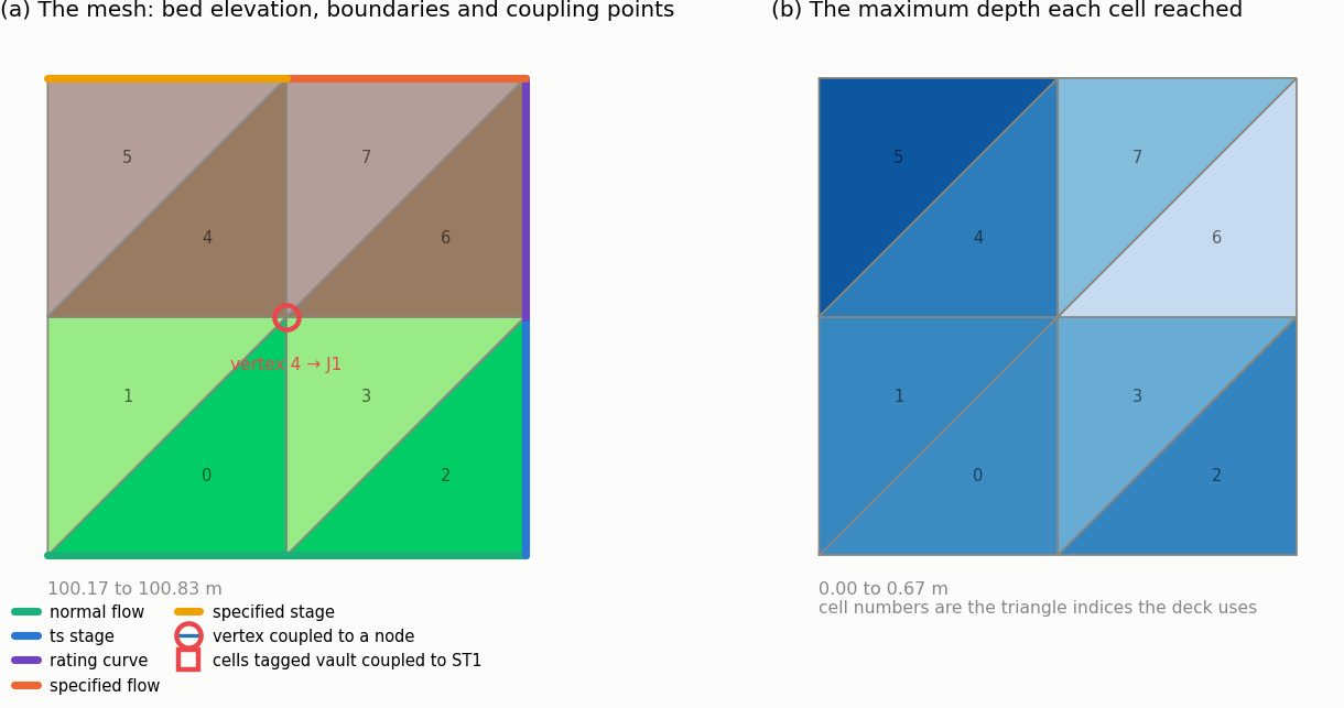
Figure 6-1 The example mesh: bed elevation, the five boundary-condition types and both kinds of coupling point

Panel (a) is the deck drawn from its own results file: the bed rises about 0.7 m from the south-west corner, the coloured perimeter segments are the five boundary types, and the circled vertex is the drain inlet mapped to node J1. Panel (b) is the maximum depth each cell reached.

The run's 2D continuity block is the first thing to read after a coupled run:

Term	Volume (m³)
Rainfall inflow	0.334
1D → 2D spill inflow	2 746.7
Boundary inflow	4 735.4
2D → 1D drain outflow	4 630.3
Boundary outflow	2 739.8
Final stored volume	112.3
Continuity error	−0.000 %

Table 6-1 The 2D Surface Routing Continuity block for this run

Both coupling directions are active: the network spills 2 747 m³ onto the surface and drains 4 630 m³ back off it. A coupled model whose spill and drain rows are both zero is not coupled, whatever its maps say — that is the first check.

Which momentum closure

Figure 6-2

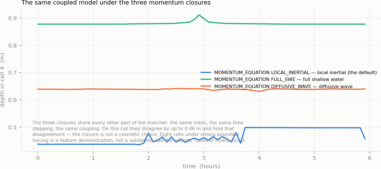
Figure 6-2 One cell's depth history under the three momentum closures

MOMENTUM_EQUATION	Peak depth in cell 4
LOCAL_INERTIAL	0.499 m
FULL_SWE	0.912 m
DIFFUSIVE_WAVE	0.642 m

Table 6-2 What each closure gives on this mesh

The three closures share everything else — the same mesh, the same time stepping, the same coupling, the same boundaries — and they disagree here by nearly half a metre, holding that disagreement through the run. The closure is not a cosmetic choice.

What this comparison is not. Eight cells under strong boundary forcing is a feature demonstration, and a spread this large on it says more about the mesh than about the closures. The place to judge them is against analytic solutions — the SWASHES cases in Hydraulics 9, §9.10 — and the guidance from those is the guidance in Chapter 1: local inertial for shallow friction-dominated spreading, full shallow water where the flow is transcritical or shocked, diffusive wave for very flat and slow water. What this figure establishes is that the choice must be made deliberately.

Where to go next

• Hydraulics 9 — the mesh, the closures, the boundary laws and the coupling formulation
• Chapter 7 — driving the same kind of mesh with rain rather than spill
• Quality 10 — carrying constituents on the mesh
• T4 — Capped Street Inlets Coupled to a 2D Surface, T3 — From a DTM to an Animated 2D Inundation Map, T5 — Culverts, Embankments, Boundary Conditions and Edge Conveyance, T6 — A Stand-alone 2D Overland-Flow Model — the same ground in the GUI
• Section: [2D_OPTIONS] and the other [2D_*] entries — the grammar of every section named here