1.1 Introduction

Urban runoff quantity and quality constitute problems of both a historical and current nature. Cities have long assumed the responsibility of control of stormwater flooding and treatment of point sources (e.g., municipal sewage) of wastewater. Since the 1960s, the severe pollution potential of urban nonpoint sources, principally combined sewer overflows and stormwater discharges, has been recognized, both through field observation and federal legislation. The advent of modern computers has led to the development of complex, sophisticated tools for analysis of both quantity and quality pollution problems in urban areas and elsewhere (Singh, 1995). The EPA Storm Water Management Model, SWMM, first developed in 1969-71, was one of the first such models. It has been continually maintained and updated and is perhaps the best known and most widely used of the available urban runoff quantity/quality models (Huber and Roesner, 2013).

SWMM is a dynamic rainfall-runoff simulation model used for single event or long-term (continuous) simulation of runoff quantity and quality from primarily urban areas. The runoff component of SWMM operates on a collection of subcatchment areas that receive precipitation and generate runoff and pollutant loads. The routing portion of SWMM transports this runoff through a system of pipes, channels, storage/treatment devices, pumps, and regulators. SWMM tracks the quantity and quality of runoff generated within each subcatchment, and the flow rate, flow depth, and quality of water in each pipe and channel during a simulation period comprised of multiple time steps.

Table 1-1 summarizes the development history of SWMM. The current edition, Version 5, is a complete re-write of the previous releases. The reference manual for this edition of SWMM is comprised of three volumes. Volume I describes SWMM's hydrologic models, Volume II its hydraulic models, and Volume III its water quality and low impact development models. These manuals complement the SWMM 5 User's Manual (US EPA, 2010), which explains how to run the program, and the SWMM 5 Applications Manual (US EPA, 2009) which presents a number of worked-out examples. The procedures described in this reference manual are based on earlier descriptions included in the original SWMM documentation (Metcalf and Eddy et al., 1971a, 1971b, 1971c, 1971d), intermediate reports (Huber et al., 1975; Heaney et al., 1975; Huber et al., 1981), plus new material. This information supersedes the Version 4.0 documentation (Huber and Dickinson, 1988; Roesner et al., 1988) and includes descriptions of some newer procedures implemented since 1988. More information on current documentation and the general status of the EPA Storm Water Management Model as well as the full program and its source code is available on the EPA SWMM web site:. http://www2.epa.gov/water-research/storm-water-management-model-swmm.

Table 1-1 Development history of SWMM

Version	Year	Contributors	Comments
SWMM I	1971	Metcalf & Eddy, Inc. Water Resources Engineers University of Florida	First version of SWMM; focus was CSO modeling; few of its methods are still used today.
SWMM II	1975	University of Florida	First widely distributed version of SWMM.
SWMM 3	1981	University of Florida Camp Dresser & McKee	Full dynamic wave flow routine, Green-Ampt infiltration, snow melt, and continuous simulation added.
SWMM 3.3	1983	US EPA	First PC version of SWMM.
SWMM 4	1988	Oregon State University Camp Dresser & McKee	Groundwater, RDII, irregular channel cross-sections and other refinements added over a series of updates throughout the 1990's.
SWMM 5	2005	US EPA CDM-Smith	Complete re-write of the SWMM engine in C; graphical user interface added; improved algorithms and new features (e.g., LID modeling) added.

1.2 SWMM's Object Model

Figure 1-1 depicts the elements included in a typical urban drainage system. SWMM conceptualizes this system as a series of water and material flows between several major environmental compartments. These compartments include:

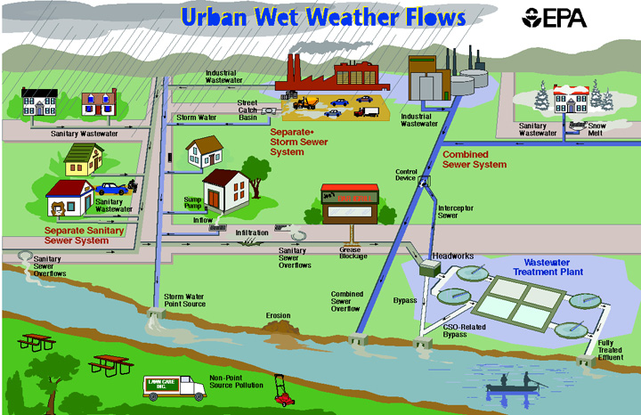
Figure 1-1 Elements of a typical urban drainage system

The Atmosphere compartment, which generates precipitation and deposits pollutants onto the Land Surface compartment.
The Land Surface compartment receives precipitation from the Atmosphere compartment in the form of rain or snow. It sends outflow in the forms of 1) evaporation back to the Atmosphere compartment, 2) infiltration into the Sub-Surface compartment and 3) surface runoff and pollutant loadings on to the Conveyance compartment.
The Sub-Surface compartment receives infiltration from the Land Surface compartment and transfers a portion of this inflow to the Conveyance compartment as groundwater interflow.
The Conveyance compartment contains a network of elements (channels, pipes, pumps, and regulators) and storage/treatment units that convey water to outfalls or to treatment facilities. Inflows to this compartment can come from surface runoff, groundwater interflow, sanitary dry weather flow, or from user-defined time series.

Not all compartments need appear in a particular SWMM model. For example, one could model just the Conveyance compartment, using pre-defined hydrographs and pollutographs as inputs. As illustrated in Figure 1-1, SWMM can be used to model any combination of stormwater collection systems, both separate and combined sanitary sewer systems, as well as natural catchment and river channel systems.

Figure 1-2 shows how SWMM conceptualizes the physical elements of the actual system depicted in Figure 1-1 with a standard set of modeling objects. The principal objects used to model the rainfall/runoff process are Rain Gages and Subcatchments. Snowmelt is modeled with Snow Pack objects placed on top of subcatchments while Aquifer objects placed below subcatchments are used to model groundwater flow. The conveyance portion of the drainage system is modeled with a network of Nodes and Links. Nodes are points that represent simple junctions, flow dividers, storage units, or outfalls. Links connect nodes to one another with conduits (pipes and channels), pumps, or flow regulators (orifices, weirs, or outlets). Land Use and Pollutant objects are used to describe water quality. Finally, a group of data objects that includes Curves, Time Series, Time Patterns, and Control Rules, are used to characterize the inflows and operating behavior of the various physical objects in a SWMM model. Table 1-2 provides a summary of the various objects used in SWMM. Their properties and functions will be described in more detail throughout the course of this manual.

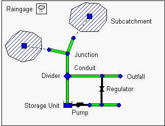
Figure 1-2 SWMM's conceptual model of a stormwater drainage system

Table 1-2 SWMM's modeling objects

Category	Object Type	Description
Hydrology	Rain Gage	Source of precipitation data to one or more subcatchments.
	Subcatchment	A land parcel that receives precipitation associated with a rain gage and generates runoff that flows into a drainage system node or to another subcatchment.
	Aquifer	A subsurface area that receives infiltration from the subcatchment above it and exchanges groundwater flow with a conveyance system node.
	Snow Pack	Accumulated snow that covers a subcatchment.
	Unit Hydrograph	A response function that describes the amount of sewer inflow/infiltration generated over time per unit of instantaneous rainfall.
Hydraulics	Junction	A point in the conveyance system where conduits connect to one another with negligible storage volume (e.g., manholes, pipe fittings, or stream junctions).
	Outfall	An end point of the conveyance system where water is discharged to a receptor (such as a receiving stream or treatment plant) with known water surface elevation.
	Divider	A point in the conveyance system where the inflow splits into two outflow conduits according to a known relationship.
	Storage Unit	A pond, lake, impoundment, or chamber that provides water storage.
	Conduit	A channel or pipe that conveys water from one conveyance system node to another.
	Pump	A device that raises the hydraulic head of water.
	Regulator	A weir, orifice or outlet used to direct and regulate flow between two nodes of the conveyance system.

Table 1-2 SWMM's modeling objects (continued)

Category	Object Type	Description
Water Quality	Pollutant	A contaminant that can build up and be washed off of the land surface or be introduced directly into the conveyance system.
	Land Use	A classification used to characterize the functions that describe pollutant buildup and washoff.
Treatment	LID Control	A low impact development control, such as a bio-retention cell, porous pavement, or vegetative swale, used to reduce surface runoff through enhanced infiltration.
	Treatment Function	A user-defined function that describes how pollutant concentrations are reduced at a conveyance system node as a function of certain variables, such as concentration, flow rate, water depth, etc.
Data Object	Curve	A tabular function that defines the relationship between two quantities (e.g., flow rate and hydraulic head for a pump, surface area and depth for a storage node, etc.).
	Time Series	A tabular function that describes how a quantity varies with time (e.g., rainfall, outfall surface elevation, etc.).
	Time Pattern	A set of factors that repeats over a period of time (e.g., diurnal hourly pattern, weekly daily pattern, etc.).
	Control Rules	IF-THEN-ELSE statements that determine when specific control actions are taken (e.g., turn a pump on or off when the flow depth at a given node is above or below a certain value).

1.3 SWMM's Process Models

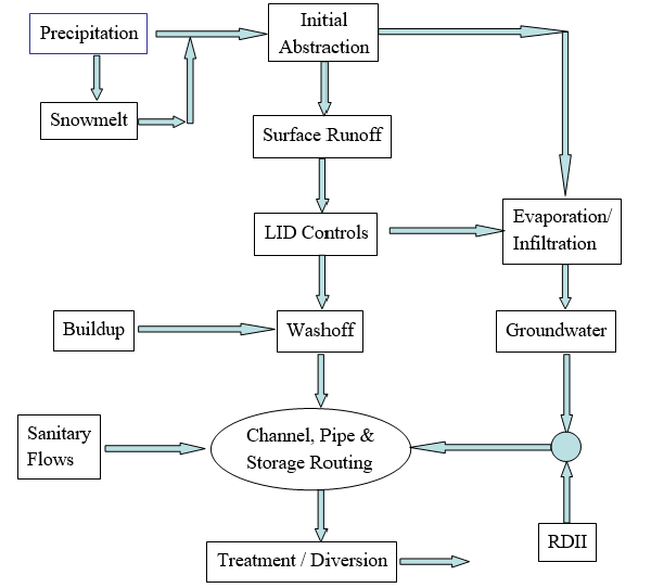
Figure 1-3 Processes modeled by SWMM

Figure 1-3 depicts the processes that SWMM models using the objects described previously and how they are tied to one another. The hydrological processes depicted in this diagram include:

time-varying precipitation
snow accumulation and melting
rainfall interception from depression storage (initial abstraction)
evaporation of standing surface water
infiltration of rainfall into unsaturated soil layers
percolation of infiltrated water into groundwater layers
interflow between groundwater and the drainage system
nonlinear reservoir routing of overland flow
infiltration and evaporation of rainfall/runoff captured by Low Impact Development controls.

The hydraulic processes occurring within SWMM's conveyance compartment include:

external inflow of surface runoff, groundwater interflow, rainfall-dependent infiltration/inflow, dry weather sanitary flow, and user-defined inflows
unsteady, non-uniform flow routing through any configuration of open channels, pipes and storage units
various possible flow regimes such as backwater, surcharging, reverse flow, and surface ponding
flow regulation via pumps, weirs, and orifices including time- and state-dependent control rules that govern their operation.

Regarding water quality, the following processes can be modeled for any number of user-defined water quality constituents:

dry-weather pollutant buildup over different land uses
pollutant washoff from specific land uses during storm events
direct contribution of rainfall deposition
reduction in dry-weather buildup due to street cleaning
reduction in washoff loads due to BMPs
entry of dry weather sanitary flows and user-specified external inflows at any point in the drainage system
routing of water quality constituents through the drainage system
reduction in constituent concentration through treatment in storage units or by natural processes in pipes and channels.

The numerical procedures that SWMM uses to model the hydrologic processes listed above are discussed in detail in subsequent chapters of this volume. SWMM's hydraulic, water quality, treatment and low impact development processes are described in subsequent volumes of this manual.

1.4 Simulation Process Overview

SWMM is a distributed discrete time simulation model. It computes new values of its state variables over a sequence of time steps, where at each time step the system is subjected to a new set of external inputs. As its state variables are updated, other output variables of interest are computed and reported. This process is represented mathematically with the following general set of equations that are solved at each time step as the simulation proceeds:

X_t = f(X_{t - 1}, I_t, P) (1-1)

Y_t = g(X_t, P) (1-2)

where

X_t = a vector of state variables at time t, Y_t = a vector of output variables at time t,

I_t = a vector of inputs at time t,

P = a vector of constant parameters,

f = a vector-valued state transition function,

g = a vector-valued output transform function.

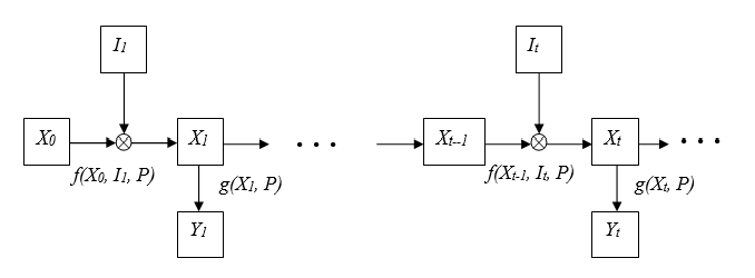
Figure 1-4 Block diagram of SWMM's state transition process

Figure 1-4 depicts the simulation process in block diagram fashion.

The variables that make up the state vector X_t are listed in Table 1-3. This is a surprisingly small number given the comprehensive nature of SWMM. All other quantities can be computed from these variables, external inputs, and fixed input parameters. The meaning of some of the less obvious state variables, such as those used for snow melt, is discussed in later chapters.

Table 1-3 State variables used by SWMM

Process	Variable	Description	Initial Value
Runoff	d	Depth of runoff on a subcatchment surface	0
Infiltration	t_p	Equivalent time on the Horton curve	0
	F_e	Cumulative excess infiltration volume	0
	F_u	Upper zone moisture content	0
	T	Time until the next rainfall event	0
	P	Cumulative rainfall for current event	0
	S	Soil moisture storage capacity remaining	User supplied
Groundwater	θ_u	Unsaturated zone moisture content	User supplied
	d_L	Depth of saturated zone	User supplied
Snowmelt	w_snow	Snow pack depth	User supplied
	f_w	Snow pack free water depth	User supplied
	a_ti	Snow pack surface temperature	User supplied
	c_c	Snow pack cold content	0
Flow Routing	y	Depth of water at a node	User supplied
	q	Flow rate in a link	User supplied
	a	Flow area in a link	Inferred from q
Water Quality	t_sweep	Time since a subcatchment was last swept	User supplied
	m_B	Mass of pollutant on subcatchment surface	User supplied
	m_P	Mass of pollutant ponded on subcatchment	0
	c_N	Concentration of pollutant at a node	User supplied
	c_L	Concentration of pollutant in a link	User supplied

*Only a sub-set of these variables is used, depending on the user's choice of infiltration method.

Examples of user-supplied input variables I_t that produce changes to these state variables include:

meteorological conditions, such as precipitation, air temperature, potential evaporation rate and wind speed
externally imposed inflow hydrographs and pollutographs at specific nodes of the conveyance system
dry weather sanitary inflows to specific nodes of the conveyance system
water surface elevations at specific outfalls of the conveyance system
control settings for pumps and regulators.

The output vector Y_t that SWMM computes from its updated state variables contains such reportable quantities as:

runoff flow rate and pollutant concentrations from each subcatchment
snow depth, infiltration rate and evaporation losses from each subcatchment
groundwater table elevation and lateral groundwater outflow for each subcatchment
total lateral inflow (from runoff, groundwater flow, dry weather flow, etc.), water depth, and pollutant concentration for each conveyance system node
overflow rate and ponded volume at each flooded node
flow rate, velocity, depth and pollutant concentration for each conveyance system link.

Regarding the constant parameter vector P, SWMM contains over 150 different user-supplied constants and coefficients within its collection of process models. Most of these are either physical dimensions (e.g., land areas, pipe diameters, invert elevations) or quantities that can be obtained from field observation (e.g., percent impervious cover), laboratory testing (e.g., various soil properties), or previously published data tables (e.g., pipe roughness based on pipe material). A smaller remaining number might require some degree of model calibration to determine their proper values. Not all parameters are required for every project (e.g., the 14 groundwater parameters for each subcatchment are not needed if groundwater is not being modeled). The subsequent chapters of this manual carefully define each parameter and make suggestions on how to estimate its value.

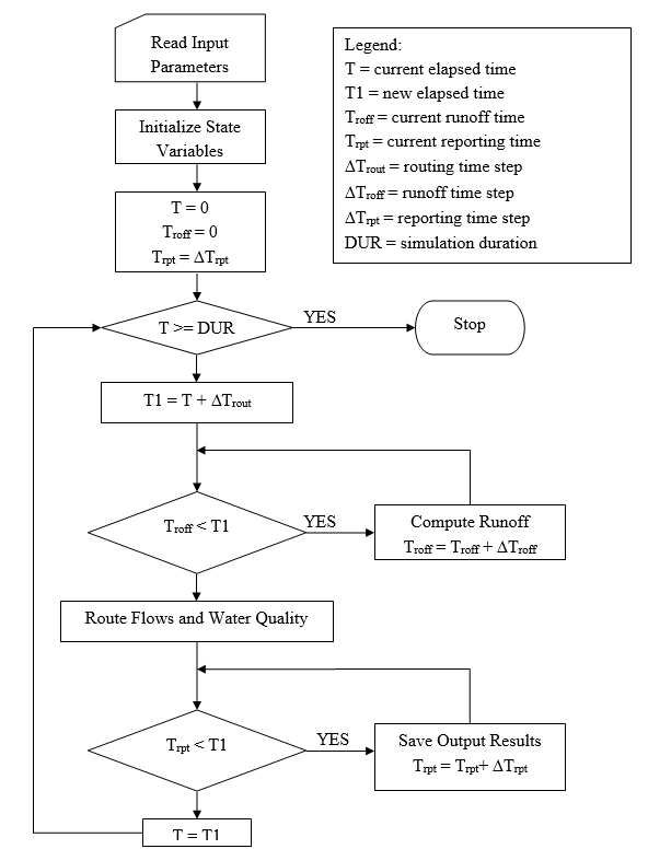
Figure 1-5 Flow chart of SWMM's simulation procedure

A flowchart of the overall simulation process is shown in Figure 1-5. The process begins by reading a description of each object and its parameters from an input file whose format is described in the SWMM 5 UsersManual (US EPA, 2010). Next the values of all state variables are initialized, as is the current simulation time (T), runoff time (T_roff), and reporting time (T_rpt).

The program then enters a loop that first determines the time T₁ at the end of the current routing time step (∆*T*_rout). If the current runoff time T_roff is less than T₁, then new runoff calculations are repeatedly made and the runoff time updated until it equals or exceeds time T₁. Each set of runoff calculations accounts for any precipitation, evaporation, snowmelt, infiltration, ground water seepage, overland flow, and pollutant buildup and washoff that can contribute flow and pollutant loads into the conveyance system.

Once the runoff time is current, all inflows and pollutant loads occurring at time T are routed through the conveyance system over the time interval from T to T₁. This process updates the flow, depth and velocity in each conduit, the water elevation at each node, the pumping rate for each pump, and the water level and volume in each storage unit. In addition, new values for the concentrations of all pollutants at each node and within each conduit are computed. Next a check is made to see if the current reporting time T_rpt falls within the interval from T to T₁. If it does, then a new set of output results at time T_rpt are interpolated from the results at times T and T₁ and are saved to an output file. The reporting time is also advanced by the reporting time step ∆*T*_rpt. The simulation time T is then updated to T₁ and the process continues until T reaches the desired total duration. SWMM's Windows-based user interface provides graphical tools for building the aforementioned input file and for viewing the computed output.

1.5 Interpolation and Units

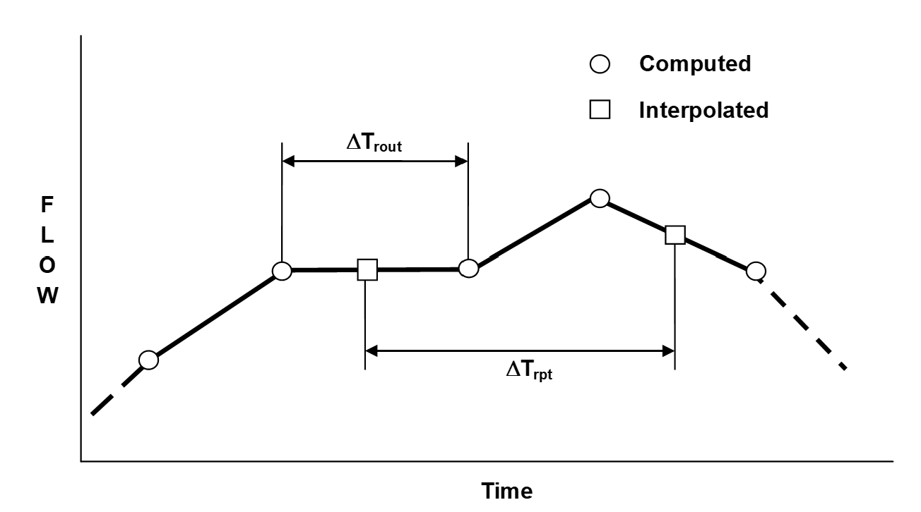
Figure 1-6 Interpolation of reported values from computed values

SWMM uses linear interpolation to obtain values for quantities at times that fall in between times at which input time series are recorded or at which output results are computed. The concept is illustrated in Figure 1-6 which shows how reported flow values are derived from the computed flow values on either side of it for the typical case where the reporting time step is larger than the routing time step. One exception to this convention is for precipitation and infiltration rates. These remain constant within a runoff time step and no interpolation is made when these values are used within SWMM's runoff algorithms or for reporting purposes. In other words, if a reporting time falls within a runoff time step the reported rainfall intensity is the value associated with the start of the runoff time step.

The units of expression used by SWMM's input variables, parameters, and output variables depend on the user's choice of flow units. If flow rate is expressed in US customary units then so are all other quantities; if SI metric units are used for flow rate then all other quantities use SI metric units. Table 1-4 lists the units associated with each of SWMM's major variables and parameters, for both US and SI systems. Internally within the computer code all calculations are carried out using feet as the unit of length and seconds as the unit of time and then converted back to the user's choice of unit system.

Table 1-4 Units of expression used by SWMM

Variable or Parameter	US Customary Units	SI Metric Units
Area (subcatchment)	acres	hectares
Area (storage surface area)	square feet	square meters
Depression Storage	inches	millimeters
Depth	feet	meters
Elevation	feet	meters
Evaporation	inches/day	millimeters/day
Flow Rate	cubic feet/sec (cfs) gallons/min (gpm) 10⁶ gallons/day (mgd)	cubic meters/sec (cms) liters/sec (lps) 10⁶ liters/day (mld)
Hydraulic Conductivity	inches/hour	millimeters/hour
Hydraulic Head	feet	meters
Infiltration Rate	inches/hour	millimeters/hour
Length	feet	meters
Manning's n	seconds/meter^1/3	seconds/meter^1/3
Pollutant Buildup	mass/acre	mass/hectare
Pollutant Concentration	milligrams/liter (mg/L) micrograms/liter (μg/L) organism counts/liter	milligrams/liter (mg/L) micrograms/liter (μg/L) organism counts/liter
Rainfall Intensity	inches/hour	millimeters/hour
Rainfall Volume	inches	millimeters
Storage Volume	cubic feet	cubic meters
Temperature	degrees Fahrenheit	degrees Celsius
Velocity	feet/second	meters/second
Width	feet	meters
Wind Speed	miles/hour	kilometers/hour

Table of Contents

1.1 Introduction

1.2 SWMM's Object Model

1.3 SWMM's Process Models

1.4 Simulation Process Overview

1.5 Interpolation and Units