 |
OpenSWMM Engine
6.0.0-alpha.4
Data-oriented, plugin-extensible SWMM Engine (6.0.0-alpha.4)
|
|
OpenSWMM Engine
6.0.0-alpha.4
Data-oriented, plugin-extensible SWMM Engine (6.0.0-alpha.4)
|
This chapter discusses how SWMM models the objects and operational parameters that constitute a stormwater drainage system. Details about how this information is entered into the program are presented in later chapters. An overview is also given on the computational methods that SWMM uses to simulate the hydrology, hydraulics and water quality behavior of a drainage system.
SWMM conceptualizes a drainage system as a series of water and material flows between several major environmental compartments. These compartments and the SWMM objects they contain include:
Not all compartments need appear in a particular SWMM model. For example, one could model just the transport compartment, using pre-defined hydrographs as inputs.
Figure 1-1 maps the compartments, the processes inside each of them and the alternative formulations OpenSWMM offers for those processes. Every alternative carries its status — Implemented, Experimental, Planned or Retired — in the same vocabulary the tables of this manual use.
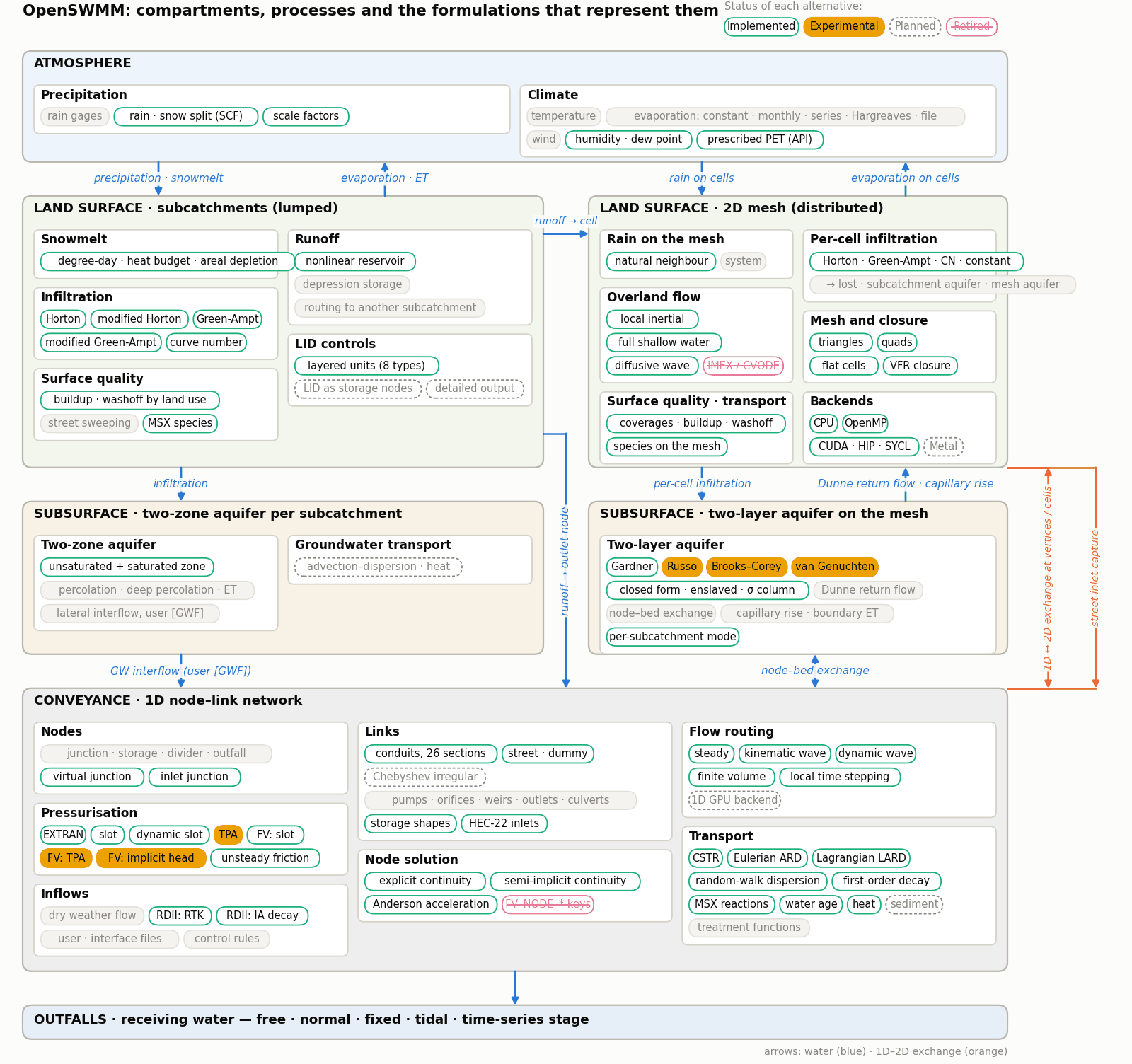
Figure 1-1 Compartments, processes and the formulations that represent them
Figure 1-2 depicts how a collection of OpenSWMM’s visual objects might be arranged together to represent a stormwater drainage system. These objects can be displayed on a map in the SWMM workspace. The following sections describe each of these objects.
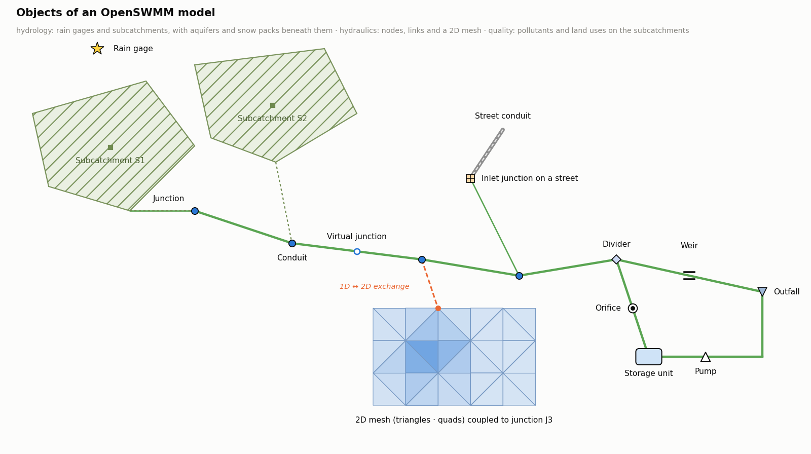
Figure 1-2 Objects of an OpenSWMM model
Rain Gages supply precipitation data for one or more subcatchment areas in a study region. The rainfall data can be either a user-defined time series or come from an external file. Several different popular rainfall file formats currently in use are supported, as well as a standard user-defined format. More details on these formats are presented in CHAPTER 3 - Files and Command-Line Operation.
The principal input properties of rain gages include:
Subcatchments are hydrologic units of land whose topography and drainage system elements direct surface runoff to a single discharge point. The user is responsible for dividing a study area into an appropriate number of subcatchments, and for identifying the outlet point of each subcatchment. Discharge outlet points can be either nodes of the drainage system or other subcatchments.
Subcatchments are divided into pervious and impervious subareas. Surface runoff can infiltrate into the upper soil zone of the pervious subarea, but not through the impervious subarea. Impervious areas are themselves divided into two subareas - one that contains depression storage and another that does not. Runoff flow from one subarea in a subcatchment can be routed to the other subarea, or both subareas can drain to the subcatchment outlet.
Infiltration of rainfall from the pervious area of a subcatchment into the unsaturated upper soil zone can be described using five different models:
To model the accumulation, re-distribution, and melting of precipitation that falls as snow on a subcatchment, it must be assigned a Snow Pack object. To model groundwater flow between an aquifer underneath the subcatchment and a node of the drainage system, the subcatchment must be assigned a set of Groundwater parameters. Pollutant buildup and washoff from subcatchments are associated with the Land Uses assigned to the subcatchment. Capture and retention of rainfall/runoff using different types of low impact development practices (such as bio-retention cells, infiltration trenches, porous pavement, vegetative swales, and rain barrels) can be modeled by assigning a set of pre-designed LID controls to the subcatchment.
The other principal input parameters for subcatchments include:
Junctions are drainage system nodes where links join together. Physically they can represent the confluence of natural surface channels, manholes in a sewer system, or pipe connection fittings. External inflows can enter the system at junctions. Excess water at a junction can become partially pressurized while connecting conduits are surcharged and can either be lost from the system or be allowed to pond atop the junction and subsequently drain back into the junction.
The principal input parameters for a junction are:
Outfalls are terminal nodes of the drainage system used to define final downstream boundaries under Dynamic Wave flow routing. For other types of flow routing they behave as a junction. Only a single link can be connected to an outfall node, and the option exists to have the outfall discharge onto a subcatchment's surface.
The boundary conditions at an outfall can be described by any one of the following stage relationships:
The principal input parameters for outfalls include:
Flow Dividers are drainage system nodes that divert inflows to a specific conduit in a prescribed manner. A flow divider can have no more than two conduit links on its discharge side. Flow dividers are only active under Steady Flow and Kinematic Wave routing and are treated as simple junctions under Dynamic Wave routing.
There are four types of flow dividers, defined by the manner in which inflows are diverted:
Cutoff Divider: diverts all inflow above a defined cutoff value. Overflow Divider: diverts all inflow above the flow capacity of the non-diverted conduit. Tabular Divider: uses a table that expresses diverted flow as a function of total inflow. Weir Divider: uses a weir equation to compute diverted flow.
The flow diverted through a weir divider is computed by the following equation
\[Q_{div} = C_W \left( f H_W \right)^{1.5} \]
where Qdiv = diverted flow, Cw = weir coefficient, Hw = weir height and f is computed as
\[f = \frac{Q_{in} - Q_{min}}{Q_{max} - Q_{min}} \]
where Qin is the inflow to the divider, Qmin is the flow at which diversion begins, and Q_max=C_W H_W^1.5. The user-specified parameters for the weir divider are Qmin, Hw, and Cw.
The principal input parameters for a flow divider are:
Storage Units are drainage system nodes that provide storage volume. Physically they could represent storage facilities as small as a catch basin or as large as a lake. The volumetric properties of a storage unit are described by a function or table of surface area versus height. In addition to receiving inflows and discharging outflows to other nodes in the drainage network, storage nodes can also lose water from surface evaporation and from seepage into native soil.
The principal input parameters for storage units include:
Conduits are pipes or channels that move water from one node to another in the conveyance system. Their cross-sectional shapes can be selected from a variety of standard open and closed geometries as listed in Table 1-1.
Most open channels can be represented with a rectangular, trapezoidal, or user-defined irregular cross-section shape. For irregular sections a Transect object is used to define how depth varies with distance across the cross-section (see CHAPTER 1 - The Conceptual Model below). Most new drainage and sewer pipes are circular while culverts typically have elliptical, rectangular or arch shapes. Elliptical and Arch pipes come in standard sizes that are listed in A7 — Reference Tables and A.13. The Filled Circular shape allows the bottom of a circular pipe to be filled with sediment and thus limit its flow capacity. The Custom Closed Shape allows any closed geometrical shape that is symmetrical about the center line to be defined by supplying a Shape Curve for the cross section (see CHAPTER 1 - The Conceptual Model below).
SWMM uses the Manning equation to express the relationship between flow rate (Q), cross-sectional area (A), hydraulic radius (R), and slope (S) in all conduits. For standard U.S. units,
\[Q = \frac{1.49}{n} A R^{2/3} S^{1/2} \]
where n is the Manning roughness coefficient. The slope S is interpreted as either the conduit slope or the friction slope (i.e., head loss per unit length), depending on the flow routing method used.
Table 1-1 Available cross section shapes for conduits Name Parameters Shape Name Parameters Shape Circular Full Height Circular Force Main Full Height, Roughness
Filled Circular Full Height, Filled Depth Rectangular - Closed Full Height, Width
Rectangular – Open Full Height, Width Trapezoidal Full Height, Base Width, Side Slopes
Triangular Full Height, Top Width Horizontal Ellipse Full Height, Max. Width
Vertical Ellipse Full Height, Max. Width Arch Full Height, Max. Width
Parabolic Full Height, Top Width Power Full Height, Top Width, Exponent
Rectangular-Triangular Full Height, Top Width, Triangle Height Rectangular-Round Full Height, Top Width, Bottom Radius
Modified Baskethandle Full Height, Bottom Width, Top Radius Egg Full Height
Horseshoe Full Height Gothic Full Height
Catenary Full Height Semi-Elliptical Full Height
Baskethandle Full Height Semi-Circular Full Height
Irregular Channel Transect Coordinates Custom Closed Shape Full Height, Shape Curve Coordinates
Street or Roadway See CHAPTER 1 - The Conceptual Model
For pipes with Circular Force Main cross-sections either the Hazen-Williams or Darcy-Weisbach formula is used in place of the Manning equation for fully pressurized flow. For U.S. units the Hazen-Williams formula is:
\[Q = 1.318\, C A R^{0.63} S^{0.54} \]
where C is the Hazen-Williams C-factor which varies inversely with surface roughness and is supplied as one of the cross-section’s parameters. The Darcy-Weisbach formula is:
\[Q = \sqrt{\frac{8g}{f}}\, A R^{1/2} S^{1/2} \]
where g is the acceleration of gravity and f is the Darcy-Weisbach friction factor. For turbulent flow, the latter is determined from the height of the roughness elements on the walls of the pipe (supplied as an input parameter) and the flow’s Reynolds Number using the Colebrook-White equation. The choice of which equation to use is a user-supplied option.
A constant rate of exfiltration of water along the length of the conduit can be modeled by supplying a Seepage Rate value (in/hr or mm/hr). This only accounts for seepage losses, not infiltration of rainfall dependent groundwater. The latter can be modeled using SWMM’s RDII feature (see CHAPTER 1 - The Conceptual Model).
A conduit can also be designated to act as a culvert (see Figure 1-4) if a Culvert Inlet Geometry code number is assigned to it. These code numbers are listed in A7 — Reference Tables. Culvert conduits are checked continuously during dynamic wave flow routing to see if they operate under Inlet Control as defined in the Federal Highway Administration’s publication Hydraulic Design of Highway Culverts Third Edition (Publication No. FHWA-HIF-12-026, April 2012). Under inlet control a culvert obeys a particular flow versus inlet depth rating curve whose shape depends on the culvert’s shape, size, slope, and inlet geometry.
Street and channel conduits with storm drain inlet structures (see Figure 1-5) use the methods described in the Federal Highway Administration's publication Urban Drainage Design Manual - HEC-22 (Publication No. FHWA-NHI-10-009, August 2013) to determine the amount of flow they capture.
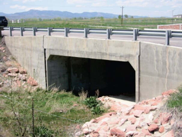
Figure 1-4 Concrete box culvert
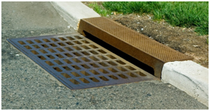
Figure 1-5 Storm drain inlet
The principal input parameters for conduits are:
Pumps are links used to lift water to higher elevations. A pump curve describes the relation between a pump's flow rate and conditions at its inlet and outlet nodes. Five different types of pump curves are supported:
Type1 (Fixed/Volume) Consists of a series of constant flow rates that apply over a series of volume intervals at the pump’s inlet node.
Type2 (Fixed/Depth) Similar to a Type1 pump except that the fixed flow rate levels vary over a set of depth intervals at the pump’s inlet node.
Type3 (Variable/Head) Uses a pump characteristic curve at some nominal impeller speed to relate flow rate and delivered head.
Type4 (Variable/Depth) A variable speed pump where flow varies continuously with inlet node water depth.
Type5 (Variable/Affinity) A variable speed version of the Type3 pump where the pump curve shifts position when control rules change the pump’s relative speed setting (see CHAPTER 1 - The Conceptual Model).
SWMM also supports an "Ideal" transfer pump that does not require a pump curve and is used mainly for preliminary analysis. Its flow rate equals the inflow rate to its inlet node no matter what the head difference is between its inlet and outlet nodes.
The on/off status of pumps can be controlled dynamically by specifying startup and shutoff water depths at the inlet node or through user-defined Control Rules. Rules can also be used to simulate variable speed drives that modulate pump flow. For a Type 5 pump, its operating curve shifts position such that flow changes in direct proportion to the controlled speed setting while head changes in proportion to the setting squared.
The principal input parameters for a pump include:
Flow Regulators are structures or devices used to control and divert flows within a conveyance system. They are typically used to:
SWMM can model the following types of flow regulators: Orifices, Weirs, and Outlets.
Orifices are used to model outlet and diversion structures in drainage systems, which are typically openings in the wall of a manhole, storage facility, or control gate. They are internally represented in SWMM as a link connecting two nodes. An orifice can have either a circular or rectangular shape, be located either at the bottom or along the side of the upstream node, and have a flap gate to prevent backflow.
Orifices can be used as storage unit outlets under all types of flow routing. If not attached to a storage unit node, they can only be used in drainage networks that are analyzed with Dynamic Wave flow routing.
The flow through a fully submerged orifice is computed as Q=CA√2gh where Q = flow rate, C = discharge coefficient, A = area of orifice opening, g = acceleration of gravity, and h = head difference across the orifice. The height of an orifice's opening can be controlled dynamically through user-defined Control Rules. This feature can be used to model gate openings and closings. Flow through a partially full orifice is computed using an equivalent weir equation.
The principal input parameters for an orifice include:
Weirs, like orifices, are used to model outlet and diversion structures in a drainage system. Weirs are typically located across a channel, along its side, or at the top of a storage unit. They are internally represented in SWMM as a link connecting two nodes, where the weir itself is placed at the upstream node. A flap gate can be included to prevent backflow.
Five varieties of weirs are available, each incorporating a different formula for computing flow across the weir as listed in Table 1-2.
Table 1-2 Available types of weirs Weir Type Cross Section Shape Flow Formula Transverse Rectangular C_W Lh^(3/2) Side flow Rectangular C_W Lh^(5/3) V-notch Triangular C_W Sh^(5/2) Trapezoidal Trapezoidal C_W Lh^(3/2)+C_WS Sh^(5/2) Roadway Rectangular C_W Lh^(3/2) Cw = weir discharge coefficient, L = weir length, S = side slope of V-notch or trapezoidal weir, h = head difference across the weir, Cws = discharge coefficient through sides of trapezoidal weir.
The Roadway weir is a broad crested rectangular weir used model roadway crossings usually in conjunction with culvert-type conduits (see Figure 1-4). It uses curves from the Federal Highway Administration publication Hydraulic Design of Highway Culverts Third Edition (Publication No. FHWA-HIF-12-026, April 2012) to determine CW as a function of h and roadway width.
Weirs can be used as storage unit outlets under all types of flow routing. If not attached to a storage unit, they can only be used in drainage networks that are analyzed with Dynamic Wave flow routing.
The height of the weir crest above the inlet node invert can be controlled dynamically through user-defined Control Rules. This feature can be used to model inflatable dams.
Weirs can either be allowed to surcharge or not. A surcharged weir will use an equivalent orifice equation to compute the flow through it. Weirs placed in open channels would normally not be allowed to surcharge while those placed in closed diversion structures or those used to represent storm drain inlet openings would be allowed to.
The principal input parameters for a weir include:
Outlets are flow control devices that are typically used to control outflows from storage units. They are used to model special head-discharge relationships that cannot be characterized by pumps, orifices, or weirs. Outlets are internally represented in SWMM as a link connecting two nodes. An outlet can also have a flap gate that restricts flow to only one direction.
Outlets attached to storage units are active under all types of flow routing. If not attached to a storage unit, they can only be used in drainage networks analyzed with Dynamic Wave flow routing.
A user-defined rating curve determines an outlet's discharge flow as a function of either the freeboard depth above the outlet's opening or the head difference across it. Control Rules can be used to dynamically adjust this flow when certain conditions exist.
The principal input parameters for an outlet include:
Map Labels were optional text annotations carried in the [LABELS] section. The engine parses the section and discards it; annotations are a concern of the graphical client, which stores its own. See 12 — Editing the Network on the Map.
In addition to physical objects that can be displayed visually on a map, SWMM utilizes several classes of non-visual data objects to describe additional characteristics and processes within a study area.
Air temperature data are used when simulating snowfall and snowmelt processes during runoff calculations. They can also be used to compute daily evaporation rates. If these processes are not being simulated then temperature data are not required. Air temperature data can be supplied to SWMM from one of the following sources:
Evaporation can occur for standing water on subcatchment surfaces, for subsurface water in groundwater aquifers, for water traveling through open channels, and for water held in storage units. Evaporation rates can be stated as:
If rates are read directly from a climate file, then a set of monthly pan coefficients should also be supplied to convert the pan evaporation data to free water-surface values. An option is also available to allow evaporation only during periods with no precipitation.
Wind speed is an optional climatic variable that is used only for snowmelt calculations. SWMM can use either a set of monthly average speeds or wind speed data contained in the same climate file used for daily minimum/maximum temperatures.
Snowmelt parameters are climatic variables that apply across the entire study area when simulating snowfall and snowmelt. They include:
Areal depletion refers to the tendency of accumulated snow to melt non-uniformly over the surface of a subcatchment. As the melting process proceeds, the area covered by snow gets reduced. This behavior is described by an Areal Depletion Curve that plots the fraction of total area that remains snow covered against the ratio of the actual snow depth to the depth at which there is 100% snow cover. A typical ADC for a natural area is shown in Figure 1-6. Two such curves can be supplied to SWMM, one for impervious areas and another for pervious areas.
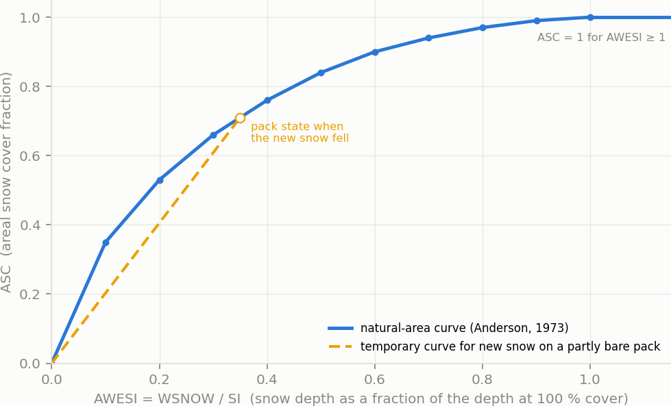
Figure 1-6 Areal depletion curve for a natural area
Climate Adjustments are optional modifications applied to the temperature, evaporation rate, and rainfall intensity that SWMM would otherwise use at each time step of a simulation. Separate sets of adjustments that vary periodically by month of the year can be assigned to these variables. They provide a simple way to examine the effects of future climate change without having to modify the original climatic time series.
A set of monthly adjustments can also be applied to the hydraulic conductivity used in computing rainfall infiltration on all pervious land surfaces, including those in all LID units, and for exfiltration from all storage nodes and conduits. These can reflect the increase of hydraulic conductivity with increasing temperature or the effect that seasonal changes in land surface conditions, such as frozen ground, can have on infiltration capacity. They can be overridden for individual subcatchments (and their LID units) by assigning a monthly infiltration adjustment Time Pattern to a subcatchment. Monthly adjustment time patterns for depression storage and pervious surface roughness coefficient (Mannings n) can also be specified for individual subcatchments
Snow Pack objects contain parameters that characterize the buildup, removal, and melting of snow over three types of subareas within a subcatchment:
Each of these three areas is characterized by the following parameters:
In addition, a set of snow removal parameters can be assigned to the Plowable area. These parameters consist of the depth at which snow removal begins and the fractions of snow moved onto various other areas.
Subcatchments are assigned a snow pack object through their Snow Pack property. A single snow pack object can be applied to any number of subcatchments. Assigning a snow pack to a subcatchment simply establishes the melt parameters and initial snow conditions for that subcatchment. Internally, SWMM creates a "physical" snow pack for each subcatchment, which tracks snow accumulation and melting for that particular subcatchment based on its snow pack parameters, its amount of pervious and impervious area, and the precipitation history it sees.
Aquifers are sub-surface groundwater zones used to model the vertical movement of water infiltrating from the subcatchments that lie above them. They also permit the infiltration of groundwater into the drainage system, or exfiltration of surface water from the drainage system, depending on the hydraulic gradient that exists. Aquifers are only required in models that need to explicitly account for the exchange of groundwater with the drainage system or to establish base flow and recession curves in natural channels and non-urban systems. The parameters of an aquifer object can be shared by several subcatchments but there is no exchange of groundwater between subcatchments. A drainage system node can exchange groundwater with more than one subcatchment.
Aquifers are represented using two zones – an un-saturated zone and a saturated zone. Their behavior is characterized using such parameters as soil porosity, hydraulic conductivity, evapotranspiration depth, bottom elevation, and loss rate to deep groundwater. In addition, the initial water table elevation and initial moisture content of the unsaturated zone must be supplied.
Aquifers are connected to subcatchments and to drainage system nodes through a subcatchment's Groundwater Flow property. This property also contains parameters that govern the rate of groundwater flow between the aquifer's saturated zone and the drainage system node.
Unit Hydrographs (UHs) estimate rainfall-dependent infiltration and inflow (RDII) into a sewer system. A UH set contains up to three such hydrographs, one for a short-term response, one for an intermediate-term response, and one for a long-term response. A UH group can have up to 12 UH sets, one for each month of the year. Each UH group is considered as a separate object by SWMM, and is assigned its own unique name along with the name of the rain gage that supplies rainfall data to it.
Each unit hydrograph, as shown in Figure 1-7, is defined by three parameters:
A unit hydrograph can also have a set of Initial Abstraction (IA) parameters associated with it. These determine how much rainfall is lost to interception and depression storage before any excess rainfall is generated and transformed into RDII flow by the hydrograph. The IA parameters consist of:
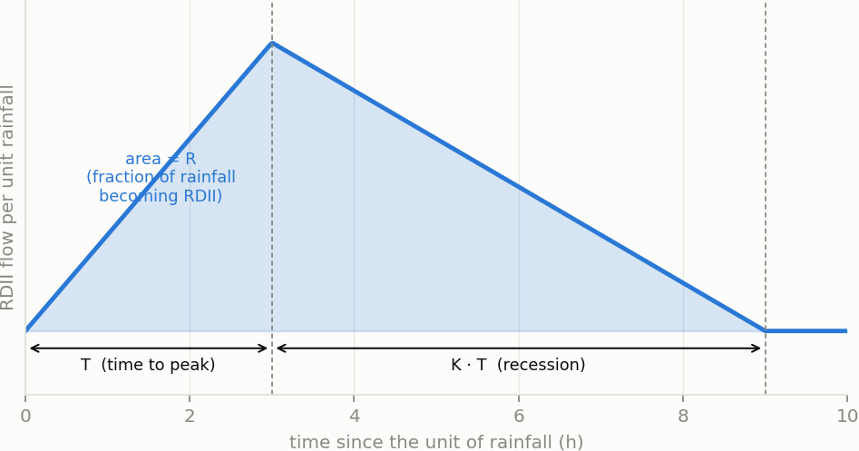
Figure 1-7 An RDII unit hydrograph
To generate RDII into a drainage system node, the node must identify (through its Inflows property) the UH group and the area of the surrounding sewershed that contributes RDII flow.
Transects refer to the geometric data that describe how bottom elevation varies with horizontal distance over the cross-section of a natural channel or irregular-shaped conduit. Figure 1-8 displays an example transect for a natural channel.
Each transect must be given a unique name. Conduits refer to that name to represent their shape. A special Transect Editor is available for editing the station-elevation data of a transect. SWMM internally converts these data into tables of area, top width, and hydraulic radius versus channel depth. In addition, as shown in Figure 1-8, each transect can have a left and right overbank section whose Manning's roughness coefficient can be different from that of the main channel. This feature can provide more realistic estimates of channel conveyance under high flow conditions.
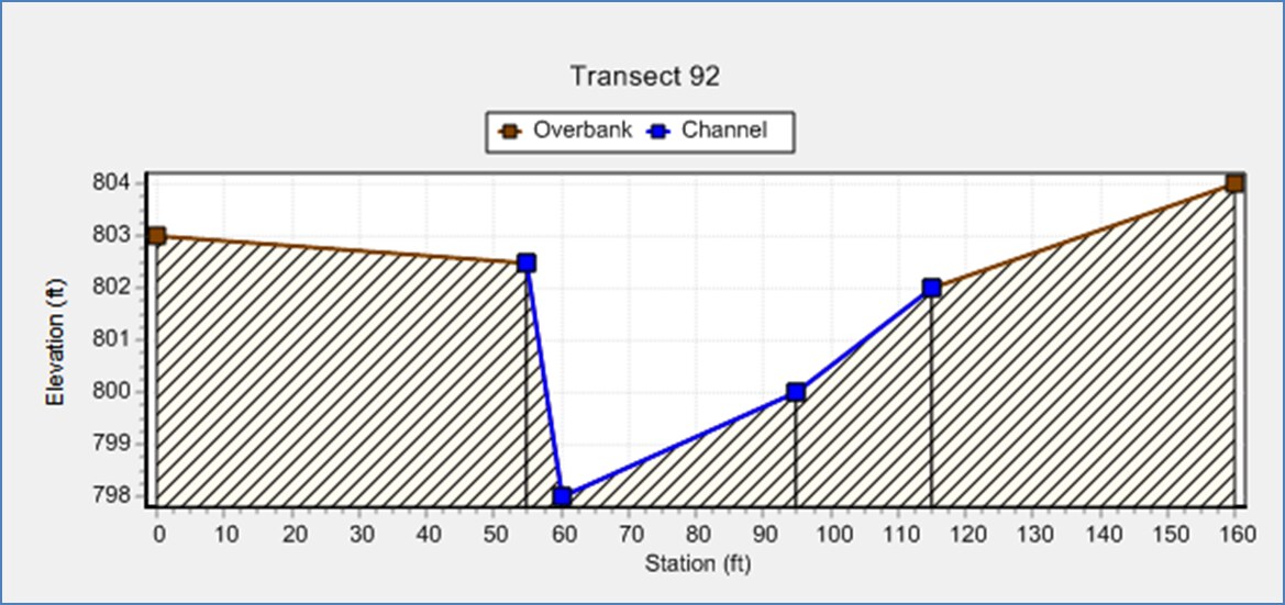
Figure 1-8 Example of a natural channel transect
Streets are a specialized form of transect that describes the typical cross-section geometry of a street or roadway. The Figure 1-9 shows a half-street layout along with the dimensions a user needs to provide.
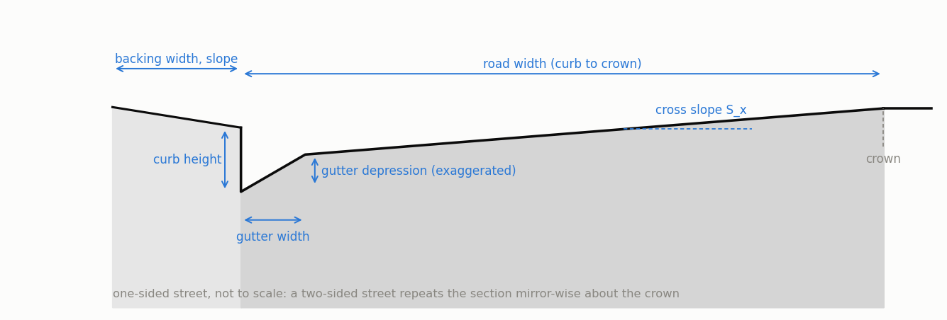
Figure 1-9 Definitional sketch of a street cross-section
Each street section object is assigned an ID name that a conduit can refer to for describing its cross-section geometry. A Street Section Editor is available for providing a street section's dimensions and whether it is one-sided or two-sided. Inlets
Street inlets are curb and gutter openings that convey runoff from streets into below-ground sewers. Drop inlets serve a similar purpose for open rectangular and trapezoidal channels. SWMM can compute the amount of flow captured by inlets and sent to designated sewer nodes using the U.S. Federal Highway Administration’s HEC-22 methodology . The type, sizing, and spacing of street inlets will determine if the spread and depth of water on roadways can be maintained at acceptable levels.
To analyze street drainage with SWMM a site is represented as a dual drainage system consisting of both street conduits along the ground surface and sewer conduits below ground (see Figure 1-10). An inlet structure will divert some portion of the street flow it carries into a designated node of the sewer system with the rest bypassed to downstream street conduits. When an inlet’s sewer node reaches its full depth any excess sewer flow that causes it to flood is routed back into the street's downstream node rather than having it leave the system as it normally would.
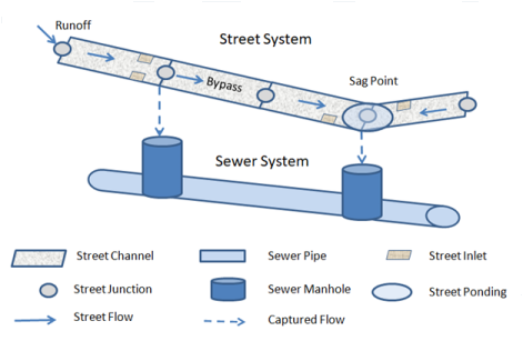
Figure 1-10 Representation of a dual drainage system
As shown in Figure 1-10, inlets can be located either on a continuous sloping section of roadway (on-grade, sometimes referred to as a flow-by condition) or at a low point where flow tends to pool (on-sag, sometimes referred to as a sump condition).
SWMM’s HEC-22 inlet capture equations support the inlet types shown in Figure 1-11. Drop inlets can only be used with open rectangular or trapezoidal channels while the other curb and gutter inlets can only be placed in conduits with Street cross-sections. An additional Custom type of inlet can be used in both streets and channels. Its capture efficiency is described by either a user-supplied Diversion curve (captured flow versus approach flow) or Rating curve (captured flow versus flow depth).
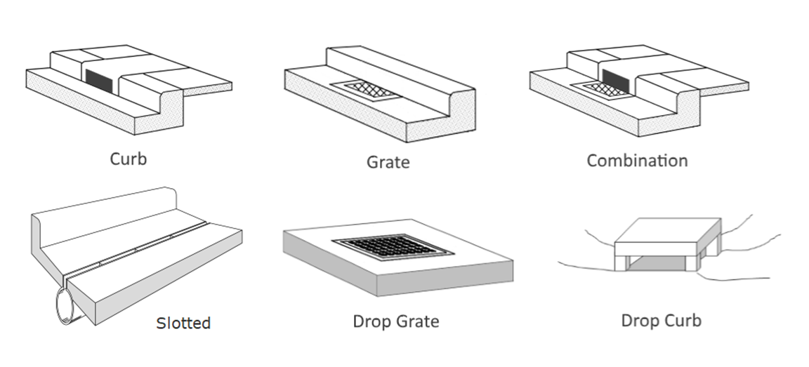
Figure 1-11 HEC-22 inlets supported by SWMM
To add an analysis of street inlets to a SWMM project:
In addition to inflows originating from subcatchment runoff and groundwater, drainage system nodes can receive three other types of external inflows:
Direct, Dry Weather, and RDII inflows are properties associated with each type of drainage system node (junctions, outfalls, flow dividers, and storage units) and can be specified when nodes are edited. They can be used to perform flow and water quality routing in the absence of any runoff computations (as in a study area where no subcatchments are defined). It is also possible to make the outflows generated from an upstream drainage system be the inflows to a downstream system by using interface files. See CHAPTER 3 - Files and Command-Line Operation for further details.
Control Rules determine how pumps and regulators in the drainage system will be adjusted over the course of a simulation. Some examples of these rules are:
Simple time-based pump control: RULE R1
IF SIMULATION TIME > 8
THEN PUMP 12 STATUS = ON
ELSE PUMP 12 STATUS = OFF
Multiple-condition orifice gate control: RULE R2A
IF NODE 23 DEPTH > 12
AND LINK 165 FLOW > 100
THEN ORIFICE R55 SETTING = 0.5
RULE R2B
IF NODE 23 DEPTH > 12
AND LINK 165 FLOW > 200
THEN ORIFICE R55 SETTING = 1.0
RULE R2C
IF NODE 23 DEPTH <= 12
OR LINK 165 FLOW <= 100
THEN ORIFICE R55 SETTING = 0
Pump station operation: RULE R3A
IF NODE N1 DEPTH > 5
THEN PUMP N1A STATUS = ON
RULE R3B
IF NODE N1 DEPTH > 7
THEN PUMP N1B STATUS = ON
RULE R3C
IF NODE N1 DEPTH <= 3
THEN PUMP N1A STATUS = OFF
AND PUMP N1B STATUS = OFF
Modulated weir height control: RULE R4 IF NODE N2 DEPTH >= 0 THEN WEIR W25 SETTING = CURVE C25
13 — Hydrology: Rain Gages, Subcatchments, LID, Snow, Groundwater and RDII describes the control rule format in more detail and the special Editor used to edit them.
SWMM can simulate the generation, inflow and transport of any number of user-defined pollutants. Required information for each pollutant includes:
Co-pollutants can also be defined in SWMM. For example, pollutant X can have a co-pollutant Y, meaning that the runoff concentration of X will have some fixed fraction of the runoff concentration of Y added to it. Pollutant buildup and washoff from subcatchment areas are determined by the land uses assigned to those areas. Input loadings of pollutants to the drainage system can also originate from external time series inflows as well as from dry weather inflows.
Land Uses are categories of development activities or land surface characteristics assigned to subcatchments. Examples of land use activities are residential, commercial, industrial, and undeveloped. Land surface characteristics might include rooftops, lawns, paved roads, undisturbed soils, etc. Land uses are used solely to account for spatial variation in pollutant buildup and washoff rates within subcatchments.
The SWMM user has many options for defining land uses and assigning them to subcatchment areas. One approach is to assign a mix of land uses for each subcatchment, which results in all land uses within the subcatchment having the same pervious and impervious characteristics. Another approach is to create subcatchments that have a single land use classification along with a distinct set of pervious and impervious characteristics that reflects the classification.
The following processes can be defined for each land use category:
Pollutant buildup that accumulates within a land use category is described (or “normalized”) by either a mass per unit of subcatchment area or per unit of curb length. Mass is expressed in pounds for US units and kilograms for metric units. The amount of buildup is a function of the number of preceding dry weather days and can be computed using one of the following functions:
Power Function: Pollutant buildup (B) accumulates proportionally to time (t) raised to some power, until a maximum limit is achieved, B=Min(C_1,C_2 t^(C_3 )) where C1 = maximum buildup possible (mass per unit of area or curb length), C2 = buildup rate constant, and C3 = time exponent.
Exponential Function: Buildup follows an exponential growth curve that approaches a maximum limit asymptotically, B=C_1 (1-e^(-C_2 t)) where C1 = maximum buildup possible (mass per unit of area or curb length) and C2 = buildup rate constant (1/days).
Saturation Function: Buildup begins at a linear rate that continuously declines with time until a saturation value is reached, B=(C_1 t)/(C_2+t) where C1 = maximum buildup possible (mass per unit area or curb length) and C2 = half-saturation constant (days to reach half of the maximum buildup).
External Time Series: This option allows one to use a Time Series to describe the rate of buildup per day as a function of time. The values placed in the time series would have units of mass per unit area (or curb length) per day. One can also provide a maximum possible buildup (mass per unit area or curb length) with this option and a scaling factor that multiplies the time series values.
Pollutant washoff from a given land use category occurs during wet weather periods and can be described in one of the following ways:
Exponential Washoff: The washoff load (W) in units of mass per hour is proportional to the product of runoff raised to some power and to the amount of buildup remaining, W=C_1 q^(C_2 ) B where C1 = washoff coefficient, C2 = washoff exponent, q = runoff rate per unit area (inches/hour or mm/hour), and B = pollutant buildup in mass units. The buildup here is the total mass (not per area or curb length) and both buildup and washoff mass units are the same as used to express the pollutant's concentration (milligrams, micrograms, or counts).
Rating Curve Washoff: The rate of washoff W in mass per second is proportional to the runoff rate raised to some power, W=C_1 Q^(C_2 ) where C1 = washoff coefficient, C2 = washoff exponent, and Q = runoff rate in user-defined flow units. Event Mean Concentration: This is a special case of Rating Curve Washoff where the exponent is 1.0 and the coefficient C1 represents the washoff pollutant concentration in mass per liter (Note: the conversion between user-defined flow units used for runoff and liters is handled internally by SWMM).
Note that in each case buildup is continuously depleted as washoff proceeds, and washoff ceases when there is no more buildup available.
Washoff loads for a given pollutant and land use category can be reduced by a fixed percentage by specifying a BMP Removal Efficiency that reflects the effectiveness of any BMP controls associated with the land use. It is also possible to use the Event Mean Concentration option by itself, without having to model any pollutant buildup at all.
Street sweeping can be used on each land use category to periodically reduce the accumulated buildup of specific pollutants. The parameters that describe street sweeping include:
Removal of pollutants from the flow streams entering any drainage system node is modeled by assigning a set of treatment functions to the node. A treatment function can be any well-formed mathematical expression involving:
The result of the treatment function can be either a concentration (denoted by the letter C) or a fractional removal (denoted by R). For example, a first-order decay expression for BOD exiting from a storage node might be expressed as: C = BOD * exp(-0.05 * HRT) where HRT is the reserved variable name for hydraulic residence time. The removal of some trace pollutant that is proportional to the removal of total suspended solids (TSS) could be expressed as: R = 0.75 * R_TSS Section C.26 provides more details on how user-defined treatment equations are supplied to the program.
Curve objects are used to describe a functional relationship between two quantities. The following types of curves are used in SWMM:
Time Series objects are used to describe how certain object properties vary with time. Time series can be used to describe:
Each time series must be given a unique name and can be assigned any number of time-value data pairs. Time can be specified either as hours from the start of a simulation or as an absolute date and time-of-day. Time series data can either be entered directly into the program or be accessed from a user-supplied Time Series file.
Time Patterns allow external Dry Weather Flow (DWF) to vary in a periodic fashion. They consist of a set of adjustment factors applied as multipliers to a baseline DWF flow rate or pollutant concentration. The different types of time patterns include: Monthly - one multiplier for each month of the year
Daily - one multiplier for each day of the week
Hourly - one multiplier for each hour from 12 AM to 11 PM
Weekend - hourly multipliers for weekend days
Each Time Pattern must have a unique name and there is no limit on the number of patterns that can be created. Each dry weather inflow (either flow or quality) can have up to four patterns associated with it, one for each type listed above. Monthly time patterns can also be used to adjust the baseline values of the following hydrological parameters:
LID Controls are low impact development practices designed to capture surface runoff and provide some combination of detention, infiltration, and evapotranspiration to it. They are considered as properties of a given subcatchment, similar to how Aquifers and Snow Packs are treated. SWMM can explicitly model eight different generic types of LID controls:
There are two different approaches for placing LID controls within a subcatchment:
The first approach allows a mix of LIDs to be placed into a subcatchment, each treating a different portion of the runoff generated from the non-LID fraction of the subcatchment. Note that under this option the subcatchment's LIDs act in parallel – it is not possible to make them act in series (i.e., have the outflow from one LID control become the inflow to another LID). Also, after LID placement the subcatchment's Percent Impervious and Width properties may require adjustment to compensate for the amount of original subcatchment area that has now been replaced by LIDs (see Figure 1-12 below). For example, suppose that a subcatchment which is 40% impervious has 75% of that area converted to a permeable pavement LID. After the LID is added the subcatchment's percent imperviousness should be changed to the percent of impervious area remaining divided by the percent of non-LID area remaining. This works out to (1 - 0.75)*40 / (100 - 0.75*40) or 14.3 %.
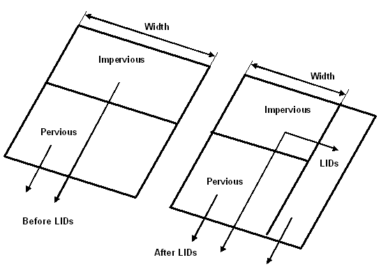
Figure 1-12 Adjustment of subcatchment parameters after LID placement
Under this first approach the runoff available for capture by the subcatchment's LIDs is the runoff generated from its impervious area. If the option to re-route some fraction of this runoff to the pervious area is exercised, then only the remaining impervious runoff (if any) will be available for LID treatment. Also note that green roofs and roof disconnection only treat the precipitation that falls directly on them and do not capture runoff from other impervious areas in their subcatchment.
The second approach allows LID controls to be strung along in series and also allows runoff from several different upstream subcatchments to be routed onto the LID subcatchment. If these single-LID subcatchments are carved out of existing subcatchments, then once again some adjustment of the Percent Impervious, Width and also the Area properties of the latter may be necessary. In addition, whenever an LID occupies the entire subcatchment the values assigned to the subcatchment's standard surface properties (such as imperviousness, slope, roughness, etc.) are overridden by those that pertain to the LID unit.
SWMM is a physically based, discrete-time simulation model. It employs principles of conservation of mass, energy, and momentum wherever appropriate. This section briefly describes the methods SWMM uses to model stormwater runoff quantity and quality through the following physical processes:
The theory and numerical methods behind each are in the three OpenSWMM reference manuals: OpenSWMM Hydrology Reference Manual, OpenSWMM Hydraulics Reference Manual and OpenSWMM Water Quality Reference Manual. Figure 1-3 shows how the processes connect, from precipitation on the subcatchments and on the 2D mesh through the subsurface to routing, transport and the outfalls.
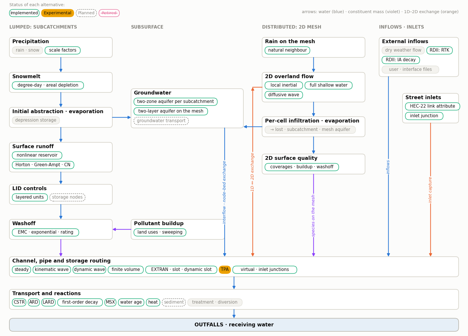
Figure 1-3 Processes modelled by OpenSWMM
The conceptual view of surface runoff used by SWMM is illustrated in Figure 1-13 below. Each subcatchment surface is treated as a nonlinear reservoir. Inflow comes from precipitation and any designated upstream subcatchments. There are several outflows, including infiltration, evaporation, and surface runoff. The capacity of this "reservoir" is the maximum depression storage, which is the maximum surface storage provided by ponding, surface wetting, and interception. Surface runoff per unit area occurs only when the depth of water in the "reservoir" exceeds the maximum depression storage, ds, in which case the outflow is given by Manning's equation. Depth of water over the subcatchment (d) is continuously updated with time by solving numerically a water balance equation over the subcatchment.
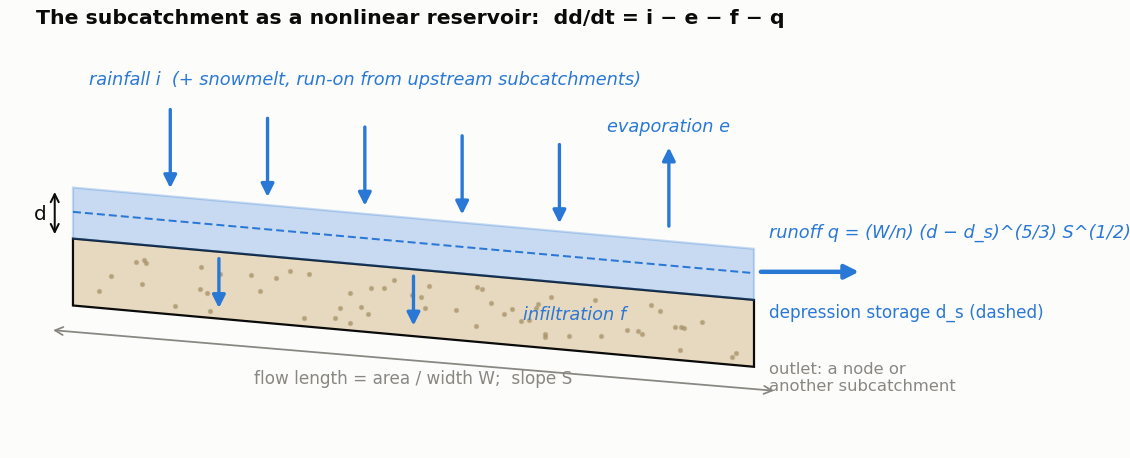
Figure 1-13 Conceptual view of surface runoff
Infiltration is the process of rainfall penetrating the ground surface into the unsaturated soil zone of pervious subcatchments areas. SWMM offers four choices for modeling infiltration:
Horton's Method This method is based on empirical observations showing that infiltration decreases exponentially from an initial maximum rate to some minimum rate over the course of a long rainfall event. Input parameters required by this method include the maximum and minimum infiltration rates, a decay coefficient that describes how fast the rate decreases over time, and a time it takes a fully saturated soil to completely dry.
Modified Horton Method This is a modified version of the classical Horton Method that uses the cumulative infiltration in excess of the minimum rate as its state variable (instead of time along the Horton curve), providing a more accurate infiltration estimate when low rainfall intensities occur. It uses the same input parameters as does the traditional Horton Method.
Green-Ampt Method This method for modeling infiltration assumes that a sharp wetting front exists in the soil column, separating soil with some initial moisture content below from saturated soil above. The input parameters required are the initial moisture deficit of the soil, the soil's hydraulic conductivity, and the suction head at the wetting front. The recovery rate of moisture deficit during dry periods is empirically related to the hydraulic conductivity.
Modified Green-Ampt Method This method modifies the original Green-Ampt procedure by not depleting moisture deficit in the top surface layer of soil during initial periods of low rainfall as was done in the original method. This change can produce more realistic infiltration behavior for storms with long initial periods where the rainfall intensity is below the soil’s saturated hydraulic conductivity.
Curve Number Method This approach is adopted from the NRCS (SCS) Curve Number method for estimating runoff. It assumes that the total infiltration capacity of a soil can be found from the soil's tabulated Curve Number. During a rain event this capacity is depleted as a function of cumulative rainfall and remaining capacity. The input parameters for this method are the curve number and the time it takes a fully saturated soil to completely dry.
SWMM also allows the infiltration recovery rate to be adjusted by a fixed amount on a monthly basis to account for seasonal variation in such factors as evaporation rates and groundwater levels. This optional monthly soil recovery pattern is specified as part of a project's Evaporation data.
Figure 1-14 is a definitional sketch of the two-zone groundwater model that is used in SWMM. The upper zone is unsaturated with a variable moisture content of . The lower zone is fully saturated and therefore its moisture content is fixed at the soil porosity . The fluxes shown in the figure, expressed as volume per unit area per unit time, consist of the following:
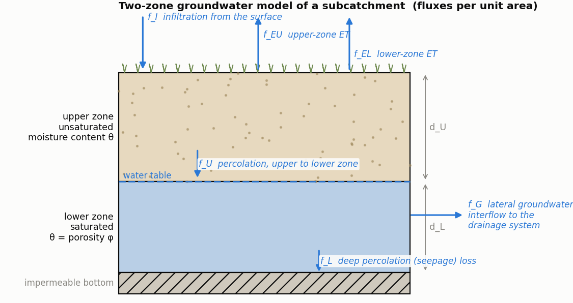
Figure 1-14 Two-zone groundwater model
fI infiltration from the surface fE evapotranspiration from the upper zone which is a fixed fraction of the un-used surface evaporation fU percolation from the upper to lower zone which depends on the upper zone moisture content and depth dU fEL evapotranspiration from the lower zone, which is a function of the depth of the upper zone dU fL seepage from the lower zone to deep groundwater which depends on the lower zone depth dL fG lateral groundwater interflow to the drainage system, which depends on the lower zone depth dL as well as the depth in the receiving channel or node.
After computing the water fluxes that exist during a given time step, a mass balance is written for the change in water volume stored in each zone so that a new water table depth and unsaturated zone moisture content can be computed for the next time step.
The snowmelt routine in SWMM is a part of the runoff modeling process. It updates the state of the snow packs associated with each subcatchment by accounting for snow accumulation, snow redistribution by areal depletion and removal operations, and snow melt via heat budget accounting. Any snowmelt coming off the pack is treated as an additional rainfall input onto the subcatchment.
At each runoff time step the following computations are made:
Flow routing within a conduit link in SWMM is governed by the conservation of mass and momentum equations for gradually varied, unsteady flow (i.e., the Saint Venant flow equations). The SWMM user has a choice on the level of sophistication used to solve these equations:
Each of these routing methods employs the Manning equation to relate flow rate to flow depth and bed (or friction) slope. For user-designated Force Main conduits, either the Hazen-Williams or Darcy-Weisbach equation can be used when pressurized flow occurs.
Steady Flow routing represents the simplest type of routing possible (actually no routing) by assuming that within each computational time step flow is uniform and steady. Thus it simply translates inflow hydrographs at the upstream end of the conduit to the downstream end, with no delay or change in shape. The normal flow equation is used to relate flow rate to flow area (or depth).
This type of routing cannot account for channel storage, backwater effects, entrance/exit losses, flow reversal or pressurized flow. It can only be used with dendritic conveyance networks, where each node has only a single outflow link (unless the node is a divider in which case two outflow links are required). This form of routing is insensitive to the time step employed and is really only appropriate for preliminary analysis using long-term continuous simulations.
This routing method solves the continuity equation along with a simplified form of the momentum equation in each conduit. The latter assumes that the slope of the water surface equal the slope of the conduit.
The maximum flow that can be conveyed through a conduit is the full normal flow value. Any flow in excess of this entering the inlet node is either lost from the system or can pond atop the inlet node and be re-introduced into the conduit as capacity becomes available.
Kinematic wave routing allows flow and area to vary both spatially and temporally within a conduit. This can result in attenuated and delayed outflow hydrographs as inflow is routed through the channel. However this form of routing cannot account for backwater effects, entrance/exit losses, flow reversal, or pressurized flow, and is also restricted to dendritic network layouts. It can usually maintain numerical stability with moderately large time steps, on the order of 1 to 5 minutes. If the aforementioned effects are not expected to be significant then this alternative can be an accurate and efficient routing method, especially for long-term simulations.
Dynamic Wave routing solves the complete one-dimensional Saint Venant flow equations and therefore produces the most theoretically accurate results. These equations consist of the continuity and momentum equations for conduits and a volume continuity equation at nodes.
With this form of routing it is possible to represent pressurized flow when a closed conduit becomes full, such that flows can exceed the full normal flow value. Flooding occurs when the water depth at a node exceeds the maximum available depth, and the excess flow is either lost from the system or can pond atop the node and re-enter the drainage system.
Dynamic wave routing can account for channel storage, backwater, entrance/exit losses, flow reversal, and pressurized flow. Because it couples together the solution for both water levels at nodes and flow in conduits it can be applied to any general network layout, even those containing multiple downstream diversions and loops. It is the method of choice for systems subjected to significant backwater effects due to downstream flow restrictions and with flow regulation via weirs and orifices. This generality comes at a price of having to use much smaller time steps, on the order of a thirty seconds or less (SWMM can automatically reduce the user-defined maximum time step as needed to maintain numerical stability).
Normally in flow routing, when the flow into a junction exceeds the capacity of the system to transport it further downstream, the excess volume overflows the system and is lost. An option exists to have instead the excess volume be stored atop the junction, in a ponded fashion, and be reintroduced into the system as capacity permits. Under Steady and Kinematic Wave flow routing, the ponded water is stored simply as an excess volume. For Dynamic Wave routing, which is influenced by the water depths maintained at nodes, the excess volume is assumed to pond over the node with a constant surface area. This amount of surface area is an input parameter supplied for the junction.
Alternatively, the user may wish to represent the surface overflow system explicitly. In open channel systems this can include road overflows at bridges or culvert crossings as well as additional floodplain storage areas. In closed conduit systems, surface overflows may be conveyed down streets, alleys, or other surface routes to the next available stormwater inlet or open channel. Overflows may also be impounded in surface depressions such as parking lots, back yards or other areas.
In sewer systems with pressurized pipes and force mains the hydraulic head at junction nodes can at times exceed the ground elevation under Dynamic Wave routing. This would normally result in an overflow which, as described above, can either be lost or ponded. SWMM allows the user to specify an additional "surcharge" depth for junction nodes that lets them pressurize and prevents any outflow until this additional depth is exceeded. If both ponding and pressurization are specified for a node ponding takes precedence and the surcharge depth is ignored. Ponding does not apply to storage nodes.
Water quality routing within conduit links assumes that the conduit behaves as a continuously stirred tank reactor (CSTR). Although a plug flow reactor assumption might be more realistic, the differences will be small if the travel time through the conduit is on the same order as the routing time step. The concentration of a constituent exiting the conduit at the end of a time step is found by integrating the conservation of mass equation, using average values for quantities that might change over the time step such as flow rate and conduit volume.
Water quality modeling within storage unit nodes follows the same approach used for conduits. For other types of nodes that have no volume, the quality of water exiting the node is simply the mixture concentration of all water entering the node.
The pollutant concentration in both a conduit and a storage node will be reduced by a first-order decay reaction if the pollutant’s first-order decay coefficient is not zero.
LID controls are represented by a combination of vertical layers whose properties are defined on a per-unit-area basis. This allows LIDs of the same design but differing area coverage to easily be placed within different subcatchments of a study area. During a simulation SWMM performs a moisture balance that keeps track of how much water moves between and is stored within each LID layer. As an example, the layers used to model a bio-retention cell and the flow pathways between them are shown in Figure 1-15. The various possible layers consist of the following:
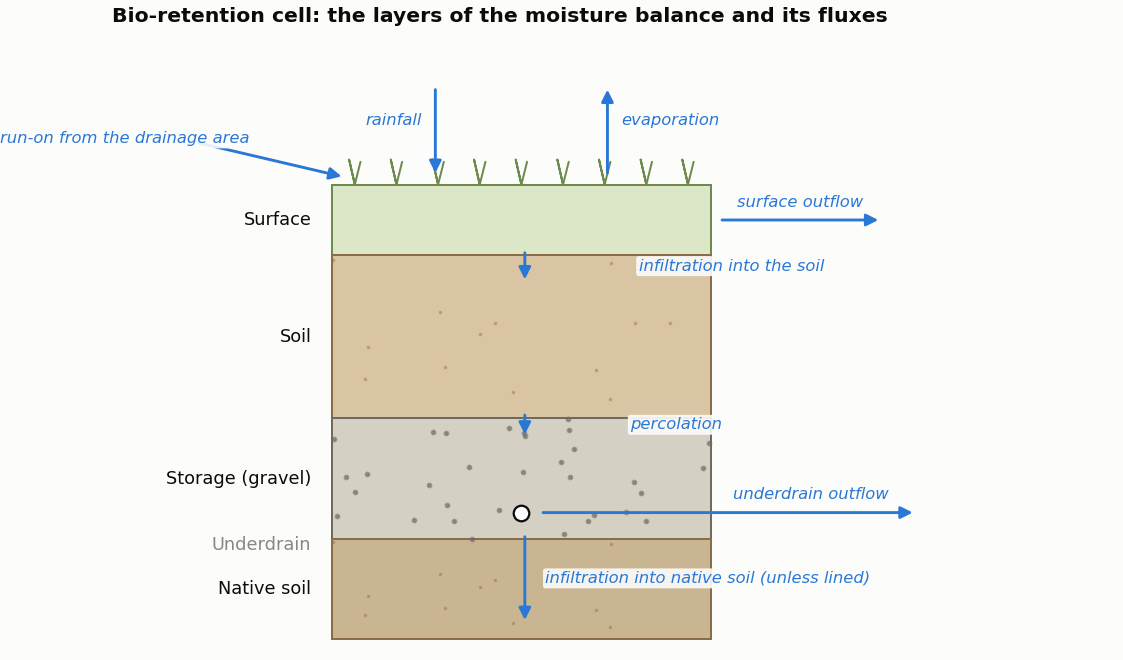
Figure 1-15 Conceptual diagram of a bio-retention cell LID
Table 1-3 Layers used to model different types of LID units LID Type Surface Pavement Soil Storage Drain Drainage Mat Bio-Retention Cell x x o o
Rain Garden x x
Green Roof x x x Permeable Pavement x x o x o
Infiltration Trench x x o
Rain Barrel x x
Roof Disconnection x x
Vegetative Swale x
All of the LID controls provide some amount of rainfall/runoff storage and evaporation of stored water (except for rain barrels). Infiltration into native soil occurs in vegetative swales and can also occur in bio-retention cells, rain gardens, permeable pavement systems, and infiltration trenches if those systems do not employ an optional impermeable bottom liner. Infiltration trenches and permeable pavement systems can also be subjected to clogging. This reduces their hydraulic conductivity over time proportional to the cumulative hydraulic loading they receive.
The performance of the LID controls placed in a subcatchment is reflected in the overall runoff, infiltration, and evaporation rates computed for the subcatchment as normally reported by SWMM. SWMM's Status Report also contains a section entitled LID Performance Summary that provides an overall water balance for each LID control placed in each subcatchment. The components of this water balance include total inflow, infiltration, evaporation, surface runoff, drain flow and initial and final stored volumes, all expressed as inches (or mm) over the LID's area. Optionally, the entire time series of flux rates and moisture levels for a selected LID control in a given subcatchment can be written to a tab delimited text file for easy viewing and graphing in a spreadsheet program (such as Microsoft Excel).
 1.13.2